Observations, Experiments, and Large Eddy Simulation

Observations, Experiments, and Large Eddy Simulation Bjorn Stevens* and Donald H. Lenschow+

ABSTRACT The authors use a 1998 workshop titled “Observations, Experiments, and Large-Eddy Simulation” as a springboard to begin a dialogue on the philosophy of simulation as well as to examine the relationship of large eddy simulation (LES) of geophysical flows to both observations and experiments. LES is shown to be perhaps the simplest representative of a broad class of activity in the geosciences, wherein the aggregated properties of fluids are solved for using approximate, or conjectural equation sets. To distinguish this type of activity from direct fluid simulation, the terms pseudofluid and pseudofluid simulation are introduced. Both direct and pseudofluid simulation introduce methodological changes into the science as they propose to provide synthetic, yet controlled, descriptions of phenomena that can then be used to help shape ideas regarding the behavior of real fluids. In this sense they differ from more traditional theoretical activities, whose goal is to provide better/simpler explanations of observed phenomena. However, because pseudofluids, by their very nature, demand testing, they supplant neither observations nor experiments. Instead they define additional opportunities and challenges for these well-established scientific methodologies. Such challenges and opportunities primarily manifest themselves as tests, which are categorized into two types: (i) tests that attempt to justify the method a priori and (ii) tests of hypotheses that are derived from the method. LES is shown to be particularly amenable to both types of tests whether they be implemented using observations or experiments. Moreover, the recent developments in laboratory and remote sensing technologies are shown to provide exciting opportunities for realizing such tests. Last, efforts to better understand LES will have peripheral benefits, both because LES shares common features with, and because LES is increasingly used as a tool to further develop, other types of pseudofluids in the geosciences. For these reasons institutional initiatives to develop symbiotic relationships between observations, experiments, and LES would be timely.

1. Introduction Numerical simulations of complex, multiscale phenomena are common in the geosciences. The everexpanding ability to perform numerical simulation, as represented by our ability to solve for the evolution

*Department of Atmospheric Sciences, University of California, Los Angeles, Los Angeles, California. + National Center for Atmospheric Research, Boulder, Colorado; The National Center for Atmospheric Research is sponsored by the National Science Foundation. Corresponding author address: Dr. Bjorn Stevens, Department of Atmospheric Sciences, University of California, Los Angeles, 405 Hilgard Ave., Box 951565, Los Angeles, CA 90095-1565. E-mail: [email protected] In final form 19 July 2000. ©2001 American Meteorological Society

Bulletin of the American Meteorological Society

of dynamical systems with millions of degrees of freedom on a desktop workstation over a weekend, introduces permanent and structural changes in the way we do science. Our capacity for numerical simulation changes how we think about reality, how we form and test ideas, and even how we organize and conduct ourselves. The influence of this developing capacity of ours is profound; but do we really understand what we are doing? Just what are these creatures we call simulations, and how do they relate to those things in our culture that are more traditional: simple models or theories, observations, and experiments. In the summers of 1997 and 1998 two workshops were organized by the Geophysical Turbulence Program (GTP) of the National Center for Atmospheric Research (NCAR) to, in part, address these issues. The first of these workshops, on Physical Reality and Numerical Simulations, dealt more philosophically with 283

the relationship between reality as perceived through familiar means (i.e., observations and experiments) and models or simulations of that reality. The second, which bore the same title as this paper (and shall hereafter be referred to either as the “OEL workshop” or simply “the OEL”), explored in a more practical manner relationships among simulations, experiments, and observations of turbulent atmospheric or oceanic boundary layers. Although this manuscript is influenced by both workshops, it draws more heavily on the subject matter of the second. Indeed, the manuscript was originally conceived as a report on the OEL workshop. Instead of simply reporting on the workshop, we decided that an article attempting to further develop the major issues that arose during the course of the workshop would be more interesting and useful. However, it is inevitable that some things that would be present in a standard report will be left out, and that the discussion will be more heavily flavored by the authors’ biases and interests. This paper is divided into two rather distinct parts. The first part (section 2) discusses the nature of simulation from a philosophical perspective. While philosophers of science have dealt extensively with methodological questions, the role and nature of simulation are only beginning to be addressed. Even then most philosophical discussions focus on climate simulation (e.g., Randall and Wielicki 1997; Shackley et al. 1998; Petersen 2000, and references therein). Thus the goal of this first part is to begin a dialog (from a practitioner’s perspective) on the philosophy of fluid simulation. The main questions we focus on are, what is simulation in general and large eddy simulation in particular, and how does it relate to observations and experiments? The second part (sections 3 and 4) draws more specifically on the deliberations of the OEL workshop, and the previously posited relationship between observations, experiments, 1 and large eddy simulation (LES). Its main conclusion is that there are two distinct types of tests of LES, both of which are readily achievable given existing technologies. In light of this, in section 4 we advocate strategic initiatives that attempt to make such tests.

1

Observations and experiments are used throughout to mean field measurements and laboratory measurements, respectively. While this is not consistent with everyone’s use of the word “experiment,” it reflects our desire to reserve the word “experiment” for those activities where control over the working fluid is maintained, and conforms to a standard dictionary definition.

284

2. Toward a philosophy of simulation Observations and experiments are longstanding, well-defined scientific endeavors. Simulation, or at least what we mean by simulation, is not. Simulation is clearly distinct from observation and experiment in that it has no explicit dependence on objective reality; that is, it is a closed theoretical exercise that at best reflects our preconceptions about reality. What is less clear is how simulation relates to other types of closed theoretical activities, and how its special characteristics might form a better basis for relating it to observation and experiment. In general scientific terms, simulation refers to the representation of the behavior or characteristics of some system, A, through the use of another system, B. Hereafter we limit our consideration primarily to real geophysical fluids (system A) and to computer programs that try to characterize their behavior (system B). Hence we use the word “simulation” synonymously with the phrases “computer simulation” or “numerical simulation.” This general definition obscures the fact that B never directly simulates A. Instead it simulates a mathematical representation, or model, of A that we denote by A′ . Introducing A′ in this matter serves the purpose of reminding us that the fidelity of any simulation depends on the fidelity of the computer program to the mathematical model (i.e., B to A′ ) and the fidelity of the model to the physical system (i.e., A′ to A). a. Minimally and maximally aggregated systems The state of any system A can be represented in a variety of ways. Consequently the model A′ , of how this state changes, can take many forms with varying degrees of similitude to A. Consider a fixed mass of gas in a cylinder. Its state can be represented in a highly aggregated fashion through the specification of its temperature and pressure, or in an essentially nonaggregated fashion through the specification of the position and momentum of each of the gas molecules. In this case we have only two degrees of freedom for the maximally aggregated system, while for the nonaggregated system there are effectively an infinite number of degrees of freedom. In both cases we arrive at model A′ that for most purposes is believed to be an acceptable model of A. As we shall see this is not always the case. The degree of aggregation of A is a distinguishing feature because our understanding of complex systems is often manifest in our ability to represent their behavior in some low-dimensional (or highly aggreVol. 82, No. 2, February 2001

gated) sense. However, to the extent that we have good mathematical models of fluid systems, such models usually correspond to essentially nonaggregated representations of the system. This situation results in a scientific strategy whereby essentially nonaggregated systems obeying readily accepted physical laws are simulated. These simulations are then analyzed with the hope of uncovering patterns, or laws, in their macroscopic or highly aggregated behavior. Such a strategy introduces methodological distinctions between minimally and maximally aggregated systems. b. Pseudofluids and real fluids In some cases the correspondence between A and A′ is effectively exact. As mentioned above, this is usually the case for essentially nonaggregated systems. In such cases we can speak of B directly simulating A and hence we can imagine ourselves simulating a real fluid. An example of such a situation is when we simulate systems (such as a weakly stirred tank of water) described by the Navier–Stokes equations at low Reynolds number (Re). Simulations of such systems are possible and are called direct numerical simulations (DNS). In principle there is no difference between an ideal laboratory experiment and its corresponding DNS. A problem arises when we consider more geophysical-like flows. In such flows the degrees of freedom in the system (as reflected say by the value of Re) are so numerous that DNS is not possible. That is, even though there exists a system A′ whose correspondence to A is effectively exact, it is for a system whose degrees of freedom are so numerous it can not be solved on a computer. To get around this difficulty we look for equations describing slightly more aggregated systems. Unfortunately such equations tend to be more conjectural, thereby breaking the correspondence between A and A′ . In such situations we speak of simulating a pseudofluid, which is a hypothetical fluid defined to correspond exactly to the mathematical system being solved A′ but whose correspondence to A cannot be considered effectively exact. In coining the term “pseudofluid” we have in mind something more specific than any equation set A′ that is conjectured to represent a real fluid. Specifically we are thinking of systems that are minimally aggregated solely for the purpose of rendering them solvable with a computer. Such systems are introduced to avail ourselves of the possibility of extending the methodological advantages of real fluid simulation to systems with too many degrees of freedom to make Bulletin of the American Meteorological Society

real fluid simulation possible. Consequently pseudofluids are methodologically distinct from simple models, or parameterization; the latter are not meant to provide us with a tool, but rather a more satisfying description of the macroscopic behavior of fluid systems. Pseudofluids also differ from these more highly aggregated models or parameterizations in that they are constructed in a fashion that preserves more of the original physics of the real fluid, and thus they tend to be more plausible descriptions of the real fluid than do more aggregated systems. To make these ideas more concrete consider the Navier–Stokes equations:

∂ ui ∂ ∂ 2 ui 1 ∂p =− +v . ui u j − ∂t ∂ xj ρ 0 ∂ xi ∂ x j ∂ x j (1)

( )

Here the state of the system is represented by the three components of velocity ui on all relevant scales. Now imagine a filter that can decompose any continuous field φ into a low-pass component φã and a residual φ′ = φ −φã. If the filter commutes with the derivative operators, then upon application to (1) it produces an equation of the form:

∂ ui ∂ 1 ∂p =− ui u j − ∂t ∂ xj ρ 0 ∂ xi

( )

+v

∂ 2 ui ∂ + ui u j − ui u j . ∂ x j∂ x j ∂ x j

[

]

(2)

This latter equation is identical in form to the original Eq. (1) except for the additional term on the rhs. This term is usually referred to as the subgrid-scale (SGS) term because physically it represents the collective effects of subgrid-scale (actually subfilter) processes on the evolution of the resolved scales (i.e., those scales unaffected by the application of the filter). In order for (2) to be solvable the SGS term must be written as a function of the resolved scales. Such a function is called an SGS model or parameterization. Exactly how one represents this SGS term is a matter of considerable debate (e.g., Meneveau and Katz 2000). The lack of a generally acceptable representation means that in the process of aggregation we have moved from a model of an essentially unaggregated system (1) that is generally believed to describe reality, to an analogous model for the aggregated sys285

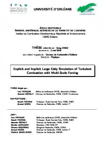
tem (2) that is on less firm ground. In terms of the above terminology, (1) describes a real fluid while (2) describes a pseudofluid. Because every set of fluid equations that we write down is actually an idealization of a real fluid, and a real fluid is itself an idealization of something even more basic, it is tempting to argue that all simulation is pseudofluid simulation. So in principle what we call DNS is simply a simulation of a Newtonian fluid, while LES is a simulation of a “Smagorinsky” fluid [at least in the case when the additional term on the rhs of Eq. (2) is modeled following Smagorinsky (1963)], where each fluid is simply a reflection of the equations being solved (Muschinski 1996). And while, in some broad philosophical sense, we do not dispute the validity of this view, we believe that the nature of the questions our community most commonly asks warrants the distinction we make. That is, the answers to most of the questions that concern us are not believed to depend on the degree of departure of real fluids from their idealization as Newtonian fluids. c. Geophysical pseudofluids and LES Geophysical examples of pseudofluid simulation range from LES to climate-system simulation. The relationship among different classes of pseudofluids, and the corresponding real fluids, is illustrated in Fig. 1. Thus, while the scales involved in precipitating deep convection range over at least 11 orders of magnitude, problems associated with the cloud-free convective boundary layer involve scales spanning at least 7 orders of magnitude. In both cases the minimally aggregated system involves so many degrees of freedom that it must be reduced to a pseudofluid involving scales spanning less than 3 orders of magnitude. The relative degree of truncation among systems necessarily depends on the degrees of freedom and the timescales in the problem at hand. Given fixed resources, simulations of more complicated systems necessarily involve synthesizing more pieces, or if you will, a greater degree of aggregation. Hence the correlation between the complexity of the parameterized physics and the proportion of explicitly represented scales in Fig. 1. LES is in some basic respects similar to other types of pseudofluid simulation (i.e., it lacks formal justification); however, it also has several distinct qualities that warrant special mention. •

Compared to other types of pseudofluids, such as GCMs and cloud-resolving models, SGS processes

286

•

•

•

in LES are relatively simple. The LES equations for cloud-free fluids have the Navier–Stokes equations as their limit as the filter scale goes to zero Many of the flows described by LES have laboratory analogs (e.g., Deardorff et al. 1980; Fedorovich et al. 1996; Fernando 1991; Sayler and Breidenthal 1998). Compared to other types of pseudofluids its use as a pseudoempirical tool is somewhat more advanced.

These factors tend to make LES, particularly for nonprecipitating flows, more amenable to a rich variety of tests. Furthermore, because LES lies at the foot of a hierarchy of pseudoflow simulations (e.g., Fig. 1), it can play a unique role in any attempt to decoct general relationships between pseudo- and real flows. 3. Observations, experiments, and LES For the reasons discussed above, we believe that the need for critical tests of LES is pressing. Fortunately many such tests are readily implemented. These points are not sufficiently recognized. LES is often compared to observations, and now and then to experiments. But as has been previously pointed out (e.g., Wyngaard 1998b) such comparisons are too often ad hoc, uncritical, and/or irrelevant. By ad hoc we mean that field observations or laboratory experiments are not typically designed specifically to test LES. Not surprisingly, such data are usually able to make only weak, qualitative statements about the fidelity of LES. By uncritical we mean that comparisons are made without clear statements as to what constitutes a significant difference (i.e., what constitutes a failure) and whether or not measurements are precise enough to show such differences. Last, by irrelevant we mean that to the extent to which they exist, corroborations of LES are rarely based on quantities that LES is looked toward as an authoritative source. That is, corroborations of LES may be based on profiles of readily measurable first- or second-order moments (e.g., Nieuwstadt et al. 1991), but then LES is used to make statements about quantities that are difficult (or impossible) to measure (e.g., Moeng and Wyngaard 1986). The OEL workshop was organized in large part because of this. The workshop participants focused on the three rather specific, albeit often overlapping, themes: scalar mixing; coherent structures; and entrainment, stratification, and wall effects. The workVol. 82, No. 2, February 2001

shop concluded with a wide-ranging discussion that we elaborate on further below. One of the more significant results of the workshop was the consolidation of the view that LES could provide a unifying framework for future research into geophysical boundary layers, but that to do so it needed to be endowed with a dual character; it needs to be seen on the one hand as a pseudofluid whose fidelity to real fluids requires further evaluation, and on the other hand as a means of generating or refining self-consistent and precise hypotheses about the behavior of real fluids. Tests of LES should reflect this dualism by either attempting to test the method in some general sense, or by testing specific physical relationships it suggests. These two types of tests and their relationship to observations and experiments are discussed below under the subject headings of method justification and hypothesis testing, respectively.2 a. Method justification Either of the following two statements (conjectures) is sufficient justification of LES. C1: The SGS model used in LES is a faithful reproduction of reality. C2: The statistics of the low-frequency modes that are explicitly calculated by LES are not sensitive to errors in the parameterization of SGS effects.

refined or calibrated. That is, in the process of testing the justification conjectures, new insight is gained that allows us to better constrain SGS models, or better define low-frequency modes, or better determine regimes in which such conjectures are well founded. Inevitably this leads to improvements in the method as a whole. 1) METHOD JUSTIFICATION AND EXPERIMENTS The strong justification conjecture (C1) for LES has been most extensively examined by the engineering community. An extensive literature on this topic has developed, particularly with regard to what are often called a priori tests of SGS models (e.g., Meneveau and Katz 2000, and references therein). Although such tests are normally made using DNS of engineering flows (e.g., Clark et al. 1979; Piomelli et al. 1997), laboratory flows can also be easily adapted to this purpose. For example, subminiature hot-wire measurements in the intermediate wake region behind a cylinder have been used to evaluate estimates of dissipation by different SGS models (O’Neil and Meneveau 1997). An important finding of this laboratory work is that even at rather large Re

Here, C1 can be considered as a strong justification conjecture and C2 as a weak justification conjecture. For this reason, and because available evidence poorly supports the first (particularly for SGS models commonly used in LES of atmospheric flows), the second is more common. Although we introduce C1 and C2 as conjectures to be tested, they can also be seen as the means through which LES is

2

A great deal can be learned simply by refining and evaluating LES by itself, either through parameter or convergence studies (e.g., Lewellen and Lewellen 1998; Bretherton et al. 1999; Mason and Brown 1999); however, we consider these sorts of tests as essential consistency checks that should be part of the normal process of forming plausible physical hypotheses on the basis of simulations, so they are not discussed further here.

Bulletin of the American Meteorological Society

FIG. 1. A rough description of the scales spanned by different phenomena and their respective pseudofluids. The x axis denotes the exponent x in a physical space scale 10x [m]. Note that some of the lines are drawn assuming that only a single decade need be resolved to exactly represent the dissipation range. The inertial range is drawn assuming turbulence production on the scale of the PBL depth (i.e., 100–1000 m). The additional scales included for flows with clouds reflect the size of cloud drops. Because a proper representation of microphysical processes requires additional variables (i.e., for the distribution of drop sizes, mixtures, etc.) estimating the degrees of freedom in the system as the cube of the ratio of the range of scales spanned by the system leads to a large underestimate. In the figure the acronyms are GCM/CSM (General Circulation/Climate System Model), MM (Mesoscale model), CRM (cloud-resolving model). 287

coherent structures appear to have a direct effect on SGS dynamics. In contrast, laboratory analogs to geophysical flows have tended to focus on the weak justification conjecture (C2), by comparing aggregated, outer-scale quantities to LES. For instance, velocity variance statistics taken from tank experiments were compared to LES of shear-free convection by Nieuwstadt et al. (1991). Similarly, measurements of entrainment rates in a variety of laboratory flow regimes (e.g., Deardorff et al. 1980; Turner and Yang 1963; McEwan and Paltridge 1976; Sayler and Breidenthal 1998; Kato and Phillips 1969; Fedorovich et al. 1996, 2000) have also been compared to LES of the corresponding regime (Sullivan et al. 1998; Stevens and Bretherton 1999). Because of the absence of such measurements, and because the results of O’Neil and Meneveau (1997) indicate a lack of universality at small scales, C1 conjectures pose an important and new class of questions for laboratory analogs to geophysical flows. Another reason for conducting further laboratory studies of surrogates for geophysical flows is the rapid pace of recent technological developments. Thermally active tracers, laser-Doppler velocimeters, laserinduced fluorescence, digital imaging of neutrally buoyant tracers, and three-dimensional holographic velocimetry allow us to ask increasingly precise questions of laboratory flows. Ultrahigh Re fluids are also now succumbing to laboratory control. Worth mentioning in this regard is the emergence of laboratory facilities that use critical Helium gas or Helium I as the working fluid (Donnelly 1998). These facilities are capable of producing flows with geophysical-like Reynolds and Rayleigh numbers (Sreenivasan 1998).3 Results from ultrahigh Re experiments are still a driving force in attempts to understand classic problems (e.g., Siggia 1994; Niemela et al. 2000) and should be employed to further address the vexing question of Re dependence. In summary, the relevance of laboratory analogs to LES and geophysical boundary layer flows, an increasingly refined theoretical context, and grand strides in laboratory technology, all argue in favor of

3

We note that DNS is also pushing the envelope to ever higher Re (e.g., Werne and Fritts 1999), albeit still orders of magnitude smaller than the state of the art experimental facilities. Nonetheless as computers become more powerful the range of scales represented by DNS and LES (e.g., Fig. 1) may, in a decade or two, begin to overlap for some problems.

288

renewed and increased support of laboratory studies of geophysical flows. 2) METHOD JUSTIFICATION AND OBSERVATIONS To our knowledge, all observationally based attempts to evaluate strong justification conjectures for LES of the PBL involve measurements in the atmospheric surface flux layer. For instance Porté-Agel et al. (1998) compared estimates of the SGS heat flux to wind and temperature measurements from a sonicanemometer placed 1.7 m above the ground. They found that traditional SGS models fail to adequately represent the data. More recently, several groups have generalized this approach to allow for a more spatially complete representation of the turbulent flow, thereby allowing one to compare aggregations of physical data that are analogous to what is implied by LES (e.g., Tong et al. 1998; Porté-Agel et al. 2000). Measurements in the atmosphere or ocean can also be brought to bear on weak justification conjectures (C2). This is important because even if attempts to corroborate SGS models in the surface flux layer are successful, the methods used are less well suited to answering similar questions in other critical parts of the flow, such as the entrainment layer. Although comparisons of LES with observational data have in the past been performed in a largely ad hoc manner they have still yielded a number of insights. For instance while normalized vertical profiles of vertical velocity variances (Lenschow et al. 1980) appear to be well represented by LES, observed profiles of vertical velocity skewness tend to be more difficult to reproduce in the simulations (Moeng and Rotunno 1990; Moyer and Young 1991). In addition differential absorption lidar (DIAL; e.g., Bösenberg 1998) measurements of top-down scalar variance in the convective boundary layer are also found to differ sharply from LES (Wulfmeyer 1999), a result that has serious implications for attempts (e.g., Kiemle et al. 1997) to use scalar variance measurements to infer entrainment velocities. Although turbulence measurements in the atmosphere are more commonplace, new technologies, such as neutrally buoyant Lagrangian floats (D’Asaro 1996), provide the potential for addressing similar issues in the ocean. Just as recent developments in laboratory measurement techniques merit renewed interest in laboratory flows, the Wulfmeyer (1999) study hints at how the increasing refinement of remote sensing technologies can be brought to bear on questions raised by LES. Because of their ability to sample a flow in more than Vol. 82, No. 2, February 2001

one dimension, and in some cases reconstruct multidimensional velocity fields, measurements from remote sensing instruments have the potential to be particularly useful for evaluating LES. For example, lidar backscatter measurements can yield important information down to a scale of a few meters about the structure of interfaces in fully developed turbulent flows—information that could conceivably be compared to previous experimental and theoretical work (e.g., Sreenivasan et al. 1989) as well as LES (e.g., Sullivan et al. 1998). More sophisticated lidar techniques (e.g., Eichinger et al. 1999, and DIAL lidars) have also been developed for measuring trace gas concentrations on scales commensurate with, or smaller than, those currently resolved by LES. These techniques, when combined with other methods such as radar Radio Acoustic Sounding System (Senff et al. 1994), or Doppler retrievals (Giez et al. 1999), provide a means for estimating fluxes remotely through the boundary layer. In addition to lidars, both cloud and clear-air radars provide a wide range of complementary capabilities that, because they sample similar flow volumes, seem well suited to evaluating LES. A disadvantage of ground-based remote sensors is their poor statistics of large-scale features (e.g., Senff et al. 1994). One way around this limitation is to mount sensors on mobile platforms (e.g., Kiemle et al. 1997); another is to make measurements over many days in relatively stationary and homogeneous conditions, and then average over similar time periods in the diurnal cycle. For example, an experiment involving Doppler lidars carried out over a period of weeks to months (to yield the highest possible number of similar days) at a site like western Utah’s salt flats (Klewicki et al. 1998) appears well suited to a critical evaluation of the ability of LES to faithfully reproduce large-scale structures in buoyancy-forced atmospheric flows. Although our focus here is on how observations can be used to test simulations, an increasingly important use of LES is to help evaluate observational techniques within what amounts to a closed theoretical system (e.g., Muschinski et al. 1999; Tong et al. 1998). b. Hypothesis testing There is a reflexive tendency to think that LES has not led to the development of any new theoretical concepts. One striking counterexample to this viewpoint (there are more) is the concept of mixed-layer scaling introduced by Deardorff (1970) on the basis of LES. However, even in this case, Deardorff developed Bulletin of the American Meteorological Society

this scaling on the basis of his numerical results combined with the insight and affirmation provided by both observational and experimental results. This is a classic example of how LES continues to be used as a tool for plying pseudo-empirical statements from the governing system of equations. In such a situation we are usually less interested in the general fidelity of LES, and more interested in whether certain key predictions of LES are correct. By using LES to frame the theoretical context for a given problem we can narrow down the parameter space and develop specific hypotheses shown to be critical to the behavior of a simpler model. This type of activity is discussed below, predominantly in the context of one specific example.4 1) ENTRAINMENT RELATIONS TO CONVECTIVE FLOWS An important question in any attempt to relate the turbulent oceanic and atmospheric PBL to parameters characterizing the larger-scale flow is, what is the entrainment rate? That is, at what rate is the nonturbulent fluid bounding the PBL eroded by the turbulence in the PBL (e.g., Phillips 1969)? In some climatologically interesting and important regions of the globe, entrainment fluxes (because of their effect on PBL cloudiness) are believed to be at least as important to the behavior of a PBL model, and the underlying coupling between the ocean and the atmosphere, as the surface fluxes (Moeng et al. 1996). Indeed, recent tests with coupled atmosphere–ocean climate models suggest that quantities ranging from the mean global radiative balance to low-frequency tropical variability are decisively sensitive to the representation of stratocumulus and by implication entrainment (Mechoso et al. 1995; Ma et al. 1996; Li and Arawaka 1999, personal communication). For these reasons, entrainment has been extensively studied using LES. Simulations of buoyancydriven PBL flows by a number of groups (e.g., Lewellen and Lewellen 1998; Lock and MacVean 1999; van Zanten et al. 1999; Moeng et al. 1999; Stevens et al. 1999b) result in entrainment velocities (we) that follow a general relationship closely related to the entrainment parameterization originally suggested by Stage and Businger (1981) on the basis of energy-balance arguments, namely,

4

In the interests of complete disclosure the authors note that they have recently been funded to do essentially what is advocated below. 289

ws3 we = α +C zml ∆b

= αws Ri −B1 + C.

(3)

(4)

Here α is a universal measure of entrainment efficiency in homogeneous buoyancy-driven flows, ws is a scale velocity related to the strength of the thermal forcing, zml is the depth of the turbulent layer, ∆b is the buoyancy jump separating the turbulent fluid from the quiescent fluid, C is an additional factor that in the cited studies accounts for undulations in the mean interface, and RiB = zml ∆b/ws2 is a bulk Richardson number. The behavior of LESs by the different groups each tend to be well constrained by the form of such a relationship. In particular one group (Lewellen and Lewellen 1998) has performed exhaustive studies of this process and found that at least in the context of their simulations such a description is remarkably robust for some regimes. Nonetheless simulations by different groups (which differ primarily in what are hoped to be algorithmic details) disagree as to the value of α, how best to define ws , and on the physical interpretation and magnitude of C. Such differences account for the approximately 30% scatter in the prediction of we among groups. Because the ensemble statistics derived from a single model tend to disperse much less than the ensemble statistics derived from a family of models, the 30% scatter among models cannot be explained as the scatter among individual flow realizations. Hence the fact that slightly different algorithms lead to simulations that seek slight but significantly different balances raises the question (e.g., Stevens et al. 1999b) as to whether the entrainment relationships that individual models seem to obey reflect physical balances, or spurious ones. Equation (3) illustrates how relationships developed through the use of LES can then go on to be tested quite independent of the simulations that inspired them. Because (3) was proposed for use in simple PBL models, all the quantities that enter into it are bulk parameters that are readily measurable. The most difficult measurement is of the entrainment rate itself (although depending on one’s interpretation of C this could also be quite difficult to measure). However measurements in nocturnal, marine stratocumulus decks should be capable of evaluating (3) to a degree of precision necessary to constrain the general behav290

ior of LES, if not to decide among the different simulations. Stratocumulus tend to be well suited for we measurements, because (i) the relationship to be tested was derived with stratocumulus in mind, (ii) they make the PBL top readily identifiable, and (iii) such layers are often relatively homogeneous. At night, the boundary layer forcing is also physically simpler to characterize, easier to measure accurately, and more stationary.5 Because C in (3) depends on the timemean structure of the interface bounding the turbulent layer, a field campaign designed to evaluate (3) must also characterize the structure of the cloud top. Entrainment relationships such as (3) are not only suited to observational corroboration. There exists an extensive literature on entrainment in laboratory flows that is largely at odds with (3)—for as yet undetermined reasons. The general consensus of the laboratory community is that the nondimensional entrainment E = we/ws scales as E ∝ Ri−Bn . In laboratory flows, with a moving grid as a source of turbulence, n is found to be either 3/2, 5/3, or 7/4 (e.g., Fernando 1991; Fernando and Hunt 1997; E and Hopfinger 1986). In convectively driven flows n is commonly taken to be unity [as is the case in Eq. (3), particularly when it is noted that C scales with Ri−B1 in both dry convective and radiatively driven flows, e.g., Sullivan et al. 1998; Moeng et al. 1999]. Further work is needed to get to the bottom of this discrepancy. For instance, investigating the relationship between entrainment scaling and the structure of the large eddies might shed some light on the source of this discrepancy, and in so doing indicate to what extent the structure of the energy containing eddies controls the overall statistics of the flow. 2) OTHER EXAMPLES We have attempted to illustrate how LES has been used to identify and craft a hypothesis, one that is central to attempts to model the interaction of the PBL with large-scale flows. Our example has been drawn

5

This latter fact, the benefit of measuring at night, illustrates our point that in the past observations and large eddy simulation were were largely independent, as virtually all simulations have been performed in the absence of solar radiative forcing, while the vast majority of all stratocumulus measurements are conducted in periods centered around local noon.

Vol. 82, No. 2, February 2001

from the workshop presentations largely because it is the one most familiar to the authors; other examples of similar importance were discussed at the OEL workshop and are adumbrated below. 1) In modeling the mean PBL structure in large-scale models one persistent question is, at what height is the presence of surface inhomogeneities no longer evident; that is, what is the blending height? M. Parlange discussed how this issue can be addressed by combining LES with lidar observations of trace gases in the convective boundary layer. Some key questions are, on what scales of surface heterogeneity is the blending concept relevant? Can temperature and passive scalars exhibit different capacities for blending? 2) A key issue in modeling the upper-ocean PBL is understanding how Langmuir circulations contribute to upper-ocean mixing (relative to wave breaking). At the OEL, E. Skyllingstad showed how key scaling parameters such as shear versus buoyancy production of turbulence and wave heights can be evaluated by LES. D’Asaro in turn suggested ways that these ideas might be tested (e.g., by evaluating the variance dissipation in different flow regimes that are expected on the basis of LES to yield widely different results) using Lagrangian floats. 3) In plume dispersion models quantitative statistics of Lagrangian dispersion are needed as a function of flow regime. Laboratory tank experiments have traditionally been used for studying dispersion. I. Sykes showed how field data could also be used to selectively test and improve LES SGS models. For instance, results from a field experiment at the Dugway Proving Ground (in Utah) reinforce previous findings (e.g., Mason and Brown 1994) and give yet another variation on what has been a consistent theme: irrespective of the flow regime LES poorly represents real flows in the surface layer. 4) A pressing question for climate simulation is, what are the ensemble statistics of fields of shallow cumulus clouds? Simulations indicate that quantities used in simple parameterizations of convection (like lateral entrainment and detrainment rates, and cloud fraction at the cloud-base level) are robust parameters of a simulation that differ by more than an order of magnitude from those commonly used in parameterizations (Siebesma and Holtslag 1996). But variables like mixing at cloud top, variance production, and cloud-top cloud fraction are found to depend much more sensitively on uncertain asBulletin of the American Meteorological Society

sumptions in the simulation (Stevens et al. 1999a). In each of these cases, answers to specific questions (in the form of LES-derived predictions) should be seen not only as “parameterization products” but clear statements that need to be tested. Clearly, many of these questions could have been framed quite independently of LES. However, we have tried to show how LES can be used to refine and sharpen questions thereby allowing much more focused observations or experiments. Of course, using LES in this manner makes the most sense in regimes where it can be shown that there is at least weak justification for its fidelity. 4. A proposal Heretofore, we have attempted to develop the background for what we believe are the two most important conclusions of the workshop. R1: Large eddy simulation provides a rich theoretical context for observations and experiments (or DNS) but supplants neither. R2: Calibrating LES and testing LES-derived hypotheses constitutes today’s leading experimental and observational challenge.6 Because the value of observations is generally not questioned, and because LES simulates many flows that have laboratory analogs, R1 essentially reaffirms the value of experiments. Here R2 goes further and states that the increasing use of LES defines a critical role for observations and experiments. However, in addition to providing measurements to help justify or refine the method, or data to test LES-derived hypotheses, we anticipate that observations and experiments will continue to play a fundamental role in the discovery of phenomena occurring in real fluids that were not initially revealed via LES. Examples of this include mesoscale convective structures revealed by, for example, satellite imagery; intermittent transport via “sweeps” and “bursts” occurring in the canopy at the surface; Langmuir circulations in the oceanic boundary layer; and decoupling of marine stratus clouds from the surface-driven turbulence layer. Once revealed, the relevant physical processes that drive these

6

Wyngaard (1998a) makes the same point but only considers what we call method justification (or calibration). 291

phenomena can then be incorporated into numerical codes and studied via LES. Given these conclusions, and the general view of LES developed throughout this manuscript, we believe that institutional initiatives that seek to better synthesize LES, observations and experiments would be timely. Moreover we have identified three principles that we believe should be incorporated into any such initiative. First, because LES stands at the nexus of several disciplines (e.g., physics, mathematics, engineering, and geosciences), any endeavor to better combine observations, experiments, and LES should strive to emphasize collaborative activity among scientists with varied backgrounds. Second, observational and experimental programs that arise from such efforts should be sharply focused toward making the best possible measurements with regard to precise questions. Experimental details, including instrument development, site location (for observational campaigns), or experimental configuration (for laboratory experiments) need to revolve around the questions being asked—more data should not be substituted for good data. Third, we note that a systematic effort will not likely be successful unless it is allowed to learn from its mistakes. Thus while such a project could (and probably should) be a temporary endeavor, it must be of sufficiently long term, and involve sufficient funding to allow the community to return to increasingly well-understood and configured field sites, or increasingly better-equipped laboratories, again and again until either the necessary measurements are made, or it is determined that they cannot be made with available resources. These respective elements, when taken together, amount to a modest proposal. In short, we are arguing that a broad community of people should be either informally or formally brought together for the purpose of better understanding LES and its relationship to large Re flows such as those commonly encountered in the atmosphere and ocean. So doing would not only bring our science to new levels of clarity, but would also provide a much stronger physical basis for some of our field’s grander endeavors—like predicting tomorrow’s weather or the next century’s climate. 5. Summary We have attempted to step back and explore the relationship of large eddy simulation to both observations and experiments. So doing required us to explore, 292

in some general sense, what is meant by simulation and how it differs from other seemingly similar activities. While we find the differences are often ones of degree, practical and aesthetic motivations warrant the categorical distinctions we make. In addition to acknowledging simulation as a distinct type of scientific activity, we further find it useful to distinguish between two types of simulation—pseudofluid simulation and real fluid simulation. The former corresponds to what is most commonly called simulation in the earth sciences, that is the solutions of a hypothetical set of equations constructed from more exact equations largely for practical reasons. The latter corresponds to the special case of solving for the time evolution of partial differential equations that are, at least for a given set of questions, widely accepted as being true. Within our categorization we have identified LES as pseudofluid simulation (i.e., it solves for the behavior of a conjecture) similar in some basic sense to climate simulation using GCMs. But in another sense LES has been identified as a prototypical pseudofluid simulation, having a particularly strong theoretical basis, well-defined limits, andz a panoply of laboratory analogs. For these reasons, and because pseudofluids of increasing complexity often incorporate statistical relations derived from simpler pseudofluids, welldesigned tests of LES stand to advance more than just our understanding of the flows that LES is conjectured to simulate. This leads us to conclude that LES cannot be used to supplant either observations or experiments, but must be used intelligently in combination with these two other activities. We outline how attempts to relate LES to experiments and observations tend to have a dual character. On one hand, observations and experiments can be used to evaluate in some a priori sense the fidelity of the LES equations. This usually amounts to an evaluation of the SGS model, but could include attempts to quantify the sensitivity of the statistics of strongly forced scales to the dynamics of the scales at which energy is dissipated. On the other hand, observations and experiments can be used to test specific conjectures developed as a result of LES. The latter activity is in a sense an indirect test of LES, but can also be seen as being independent of LES. Examples of how experiments, observations, and LES can be combined are drawn from the deliberations of the OEL workshop and suggest that more concerted efforts could yield considerable insights. Overall, our conclusions mirror the recommendations of the OEL workshop and motivate a proposal that states that Vol. 82, No. 2, February 2001

mechanisms for a better synthesis of observations, experiments, and LES need to be developed. Such mechanisms can be encouraged by institutional initiatives that emphasize collaboration, focus, and persistence. Acknowledgments. This paper was motivated by a desire to give a creative report on a 1998 summer workshop, bearing the same title as this paper, that was sponsored by the Geophysical Turbulence Program (GTP) at the National Center for Atmospheric Research (NCAR). We thank our coorganizers, and the participants, many of whom may recognize their ideas herein, albeit in a filtered form. Two other workshops also helped motivate this manuscript, one titled “Physical Reality and Numerical Simulations” was organized by GTP in 1997, the other titled “Lidars, RASS, LES, and Climate: What’s the Connection” was organized by the remote sensing group at the Max Planck Institute for Meteorology in Hamburg, Germany, in the spring of 1999. Adam Sobel is thanked for his many substantive criticisms of very preliminary drafts. Tom Horst, Dave Lewellen, Doug Lilly, Charles Meneveau, Chin-Hoh Moeng, Andreas Muschinski, Marc Parlange, Arthur Petersen, Jeffrey Weil, and John Wyngaard also provided valuable suggestions. B. Stevens acknowledges support from the Alexander von Humboldt Foundation and NSF Grant ATM-9985413. NSF is also thanked for its support of the GTP sponsored workshops, both through its funding of NCAR, and through its funding of special travel stipends for young scientists.

References Bösenberg, J., 1998: Ground-based differential absorption lidar for water-vapor and temperature profiling: Methodology. Appl. Opt., 37, 3845–3860. Bretherton, C. S., and Coauthors, 1999: An intercomparison of radiatively-driven entrainment and turbulence in a smoke cloud, as simulated by different numerical models. Quart. J. Roy. Meteor. Soc., 125, 391–423. Clark, R. A., J. H. Ferziger, and W. C. Reynolds, 1979: Evaluation of subgrid-scale models using an accurately simulated turbulent flow. J. Fluid Mech., 91, 1–16. D’Asaro, E. A., 1996: A Lagrangian float. J. Atmos. Oceanic Technol., 13, 1230–1246. Deardorff, J. W., 1970: Convective velocity and temperature scales for the unstable planetary boundary layer and for Rayleigh convection. J. Atmos. Sci., 27, 1211–1213. ——, G. E. Willis, and B. H. Stockton, 1980: Laboratory studies of the entrainment zone of a convectively mixed layer. J. Fluid Mech., 100, 41–64. Donnelly, R. J., 1998: Ultra-high Reynolds number flows using cryogenic Helium: An overview. Flow at Ultra-High Reynolds and Rayleigh Numbers: A Status Report, R. J. Donnelly and K. R. Sreenivasan, Eds., Springer, 1–29. E, X., and E. J. Hopfinger, 1986: On mixing across an interface in stably stratified fluid. J. Fluid Mech., 166, 227–244. Eichinger, W. E., D. I. Cooper, P. R. Forman, J. Griegos, M. A. Osborn, D. Richter, L. L. Tellier, and R. Thornton, 1999: The development of a scanning Raman water vapor lidar for boundary layer and tropospheric observations. J. Atmos. Oceanic

Bulletin of the American Meteorological Society

Technol., 16, 1753–1766. Fedorovich, E., R. Kaiser, M. Rau, and E. Plate, 1996: Wind tunnel study of turbulent flow structure in the convective boundary layer capped by a temperature inversion. J. Atmos. Sci., 53, 1273–1289. ——, F. T. M. Nieuwstadt, and R. Kaiser, 2000: Numerical and laboratory study of horizontally evolving convective boundary layer. Part I: Transition regimes and development of the mixed layer. J. Atmos. Sci., in press. Fernando, H. J. S., 1991: Turbulent mixing in stratified fluids. Ann. Rev. Fluid Mech., 23, 455–493. ——, and J. C. R. Hunt, 1997: Turbulence, waves and mixing at shear-free density interfaces. Part 1. A theoretical model. J. Fluid Mech., 347, 197–234. Giez, A., G. Ehret, R. Schwiesow, K. J. Davis, and D. H. Lenschow, 1999: Water vapor flux measurements from ground-based vertically pointed water vapor differential absorption and Doppler lidars. J. Atmos. Oceanic Technol., 16, 237–250. Kato, H., and O. M. Phillips, 1969: On the penetration of the turbulent layer into a stratified fluid. J. Fluid Mech., 37, 643– 665. Kiemle, C., G. Ehret, A. Giez, K. J. Davis, D. H. Lenschow, and S. P. Oncley, 1997: Estimation of boundary-layer humidity fluxes and statistics from airborne DIAL. J. Geophys. Res., 102, 29 189–29 203. Klewicki, J. C., J. F. Foss, and J. M. Wallace, 1998: High Reynolds number boundary layer turbulence in the atmospheric surface layer above western Utah’s salt flats. Flow at Ultra-High Reynolds and Rayleigh Numbers: A Status Report, R. J. Donnelly and K. R. Sreenivasan, Eds., Springer, 466 pp. Lenschow, D. H., J. C. Wyngaard, and W. T. Pennell, 1980: Meanfield and second-moment budgets in a baroclinic, convective boundary layer. J. Atmos. Sci., 37, 1314–1326. Lewellen, D., and W. Lewellen, 1998: Large-eddy boundary layer entrainment. J. Atmos. Sci., 55, 2645–2665. Lock, A. P., and M. K. MacVean, 1999: A parametrization of entrainment driven by surface heating and cloud-top cooling. Quart. J. Roy. Meteor. Soc., 125, 271–300. Ma, C.-C., C. R. Mechoso, A. W. Robertson, and A. Arakawa, 1996: Peruvian stratus clouds and the tropical Pacific circulation. J. Climate, 9, 1635–1645. Mason, P., and A. R. Brown, 1994: The sensitivity of large-eddy simulations of turbulent shear flow to subgrid models. Bound.Layer Meteor., 70, 133–150. ——, and ——, 1999: On subgrid models and filter operations in large eddy simulations. J. Atmos. Sci., 56, 2101–2114. McEwan, A. D., and G. W. Paltridge, 1976: Radiatively driven thermal convection bounded by an inversion—A laboratory simulation of stratus clouds. J. Geophys. Res., 81, 1095–1102. Mechoso, C. R., and Coauthors, 1995: The seasonal cycle over the tropical Pacific in coupled ocean–atmosphere general circulation models. Mon. Wea. Rev., 123, 2825–2838. Meneveau, C., and J. Katz, 2000: Scale-invariance and turbulence models for large-eddy simulation. Annual Review of Fluid Mechanics, J. L. Lumley, M. van Dycke, and H. L. Reed, Eds., Vol. 32, Annual Reviews Inc., 1–32. Moeng, C.-H., and J. C. Wyngaard, 1986: An analysis of closures for pressure-scalar covariances in the convective boundary layer. J. Atmos. Sci., 43, 2499–2513.

293

——, and R. Rotunno, 1990: Vertical-velocity skewness in the buoyancy-driven boundary layer. J. Atmos. Sci., 47, 1149– 1162, ——, and Coauthors, 1996: Simulation of a stratocumulus-topped PBL: Intercomparison among different numerical codes. Bull. Amer. Meteor. Soc., 77, 261–278. ——, P. P. Sullivan, and B. Stevens, 1999: Including radiative effects in an entrainment rate formula for buoyancy-driven PBLs. J. Atmos. Sci., 56, 1031–1049. Moyer, K. A., and G. S. Young, 1991: Observations of vertical velocity skewness within the marine stratocumulus-topped boundary layer. J. Atmos. Sci., 48, 403–410. Muschinski, A., 1996: A similarity theory of locally homogeneous and isotropic turbulence generated by a Smagorinsky-type LES. J. Fluid Mech., 325, 239–260. ——, P. P. Sullivan, D. B. Wuertz, R. Hill, S. A. Cohn, D. H. Lenschow, and D. J. Doviak, 1999: First synthesis of windprofiler signals on the basis of large-eddy simulation data. Radio Sci., 34, 1437–1459. Niemela, J. J., L. Skrbek, K. Sreenivasan, and R. J. Donnelly, 2000: Turbulent convection at very high Rayleigh numbers. Nature, 404, 837–840. Nieuwstadt, F. T. M., P. J. Mason, C. H. Moeng, and U. Schumann, 1991: Large-eddy simulation of the convective boundary layer: A comparison of four computer codes. Selected Papers from the 8th Symposium on Turbulent Shear Flows, F. Durst, Ed., Springer-Verlag, 343–367. O’Neil, J., and C. Meneveau, 1997: Subgrid-scale stresses and their modelling in a turbulent plane wake. J. Fluid Mech., 349, 253–293. Petersen, A. C., 2000: Philosophy of climate science. Bull. Amer. Meteor. Soc., 81, 265–271. Phillips, O. M., 1969: The Dynamics of the Upper Ocean. Cambridge University Press, 261 pp. Piomelli, U., G. N. Coleman, and J. Kim, 1997: On the effects of nonequilibrium on the subgrid-scale stresses. Phys. Fluids., 9, 2740–2748. Porté-Agel, F., C. Meneveau, and M. B. Parlange, 1998: Some basic properties of the surrogate subgrid-scale heat flux in the atmospheric boundary layer. Bound.-Layer Meteor., 88, 425– 444. ——, ——, ——, W. E. Eichinger, and M. Pahlow, 2000: Subgridscale dissipation in the atmospheric surface layer: Effects of stability and filter dimension. J. Hydrometeor., 1, 75–87. Randall, D. A., and B. A. Wielicki, 1997: Measurements, models, and hypotheses in the atmospheric sciences. Bull. Amer. Meteor. Soc., 78, 399–406. Sayler, B. J., and R. E. Bridenthal, 1998: Laboratory simulations of radiatively induced entrainment in stratiform clouds. J. Geophys. Res., 103 (D8), 8827–8837. Senff, C., J. Bösenberg, and G. Peters, 1994: Measurement of water vapor flux profiles in the convective boundary layer with lidar and radar-RASS. J. Atmos. Oceanic Technol., 11, 85–93. Shackley, S., P. Young, S. Parkinson, and B. Wynne, 1998: Uncertainty, complexity and concepts of good science in climate change modeling: Are GCMs the best tools? Climatic Change, 38, 155–201.

294

Siebesma, A. P., and A. A. M. Holtslag, 1996: Model impacts of entrainment and detrainment in shallow cumulus convection. J. Atmos. Sci., 53, 2354–2364. Siggia, E. D., 1994: High Rayleigh number convection. Annual Review of Fluid Mechanics, J. L. Lumley, M. van Dycke, and H. L. Reed, Eds., Vol. 26, Annual Reviews Inc., 137–168. Smagorinsky, J., 1963: General circulation experiments with the primitive equations. Mon. Wea. Rev., 91, 99–164. Sreenivasan, K. R., 1998: Helium flows at ultra-high Reynolds and Rayleigh numbers. Flow at Ultra-High Reynolds and Rayleigh Numbers: A Status Report, R. J. Donnely and K. R. Sreenivasan, Eds., Springer, 29–51. ——, R. Ramshankar, and C. Meneveau, 1989: Mixing, entrainment and fractal dimensions of surfaces in turbulent flows. Proc. Roy. Soc. London, 421A, 79–108. Stage, S. A., and J. A. Businger, 1981: A model for entrainment into a cloud-topped marine boundary layer. Part I: Model description and application to a cold-air outbreak episode. J. Atmos. Sci., 38, 2213–2229. Stevens, B., and Coauthors, 1999a: Cloud fraction and trade cumulus: An LES intercomparison study. Preprints, 13th Symp. on Boundary Layers and Turbulence, Dallas, TX, Amer. Meteor. Soc., 267–270. ——, C.-H. Moeng, and P. P. Sullivan, 1999b: Large-eddy simulations of radiatively driven convection: Sensitivities to the representation of small scales. J. Atmos. Sci., 56, 3963–3984. Stevens, D., and C. S. Bretherton, 1999: Effects of resolution on the simulation of stratocumulus entrainment. Quart. J. Roy. Meteor. Soc., 125, 425–439. Sullivan, P., C.-H. Moeng, B. Stevens, D. H. Lenschow, and S. D. Mayor, 1998: Entrainment and structure of the inversion layer in the convective planetary boundary layer. J. Atmos. Sci., 55, 3042–3064. Tong, C., J. C. Wyngaard, S. Khanna, and J. G. Brasseur, 1998: Resolvable- and subgrid-scale measurement in the atmospheric surface layer: Technique and issues. J. Atmos. Sci., 55, 3114– 3126. Turner, J. S., and I. K. Yang, 1963: Turbulent mixing at the top of stratocumulus clouds. J. Fluid Mech., 17, 212–224. van Zanten, M. C., P. G. Duynkerke, and J. W. M. Cuijpers, 1999: Entrainment parameterization in convective boundary layers derived from large eddy simulations. J. Atmos. Sci., 56, 813– 828. Werne, J., and D. C. Fritts, 1999: Stratified shear turbulence: Evolution and statistics. Geophys. Res. Lett., 26, 439–442. Wulfmeyer, V., 1999: Investigations of humidity skewness and variance profiles in the convective boundary layer and comparison of the latter with large eddy simulation results. J. Atmos. Sci., 56, 1077–1087. Wyngaard, J. C., 1998a: Boundary-layer modeling: History, philosophy and sociology. Clear and Cloudy Boundary Layers, A. A. M. Holtslag and P. G. Duynkerke, Eds., Elsevier, 325– 332. ——, 1998b: Experiment, numerical modeling, numerical simulation, and their roles in the study of convection. Buoyant Convection in Geophysical Flows, E. J. Plate et al., Eds., Vol. 513 of C, Kluwer, 239–251.

Vol. 82, No. 2, February 2001