subset of the state vector of linear time-invariant multivariable dynamic ..... is able to estimate the corresponding states and provide them to the controller 30 for ...
Observing a subset of the states of linear systems M. Aldeen H. Trinh
Indexing terms: Linear networks, Modelling, Dynamic systems
Abstract: A selective state observer capable of asymptotically tracking any arbitrarily chosen subset of the state vector of linear time-invariant multivariable dynamic systems is introduced. The dynamics of the observer are derived from a model of the subset to be estimated. It is shown that the only condition for the asymptotic tracking of the subset is that the derived model be observable. A simple and systematic observer design method is presented and numerical examples are given to illustrate the properties of the new observer and its design method. L i s t of symbols
x U
y
A B C
x, x2
A, Bi C, ii K,
F, A4 m(i,j) z
2
= n-dimensional state vector = r-dimensional control input vector = m-dimensional output vector = (n x n) real constant matrix = (n x r ) real constant matrix
= (m x n) real constant matrix = n, subset of x = n 2 = (n - n,) subset of x = (nix nj) real constant matrices; i, j = 1, 2 = (nix r ) real constant matrices; i = 1, 2 = (m x ni)real constant matrices; i = 1 , 2 = dxJdt;i =
1,2
= ith subsystem observer gain matrix = ith subsystem controller gain matrix = (n x n) modal transformation matrix = Ij'th element of M ; i, j = 1,2, . . . , n = n state vector = ni subset of z ; i = 1,2 = diag (Al,. . . , in)
Aii
= (nix
A: E: C:
= (n,x
ni)submatrix of A; i = 1 , 2
r = (n x r) complex matrix Ti = (ni x r) complex submatrix of r; i = 1,2 r(j,k) = jkth element of r ; j = 1, 2, ..., n ; k = 1,2, ..., r Df
ni) constant real matrix; i = 1, 2 = (ni x r) constant real matrix; i = 1 , 2 = (m x ni) constant real matrix; i = 1, 2 = (m x r) constant real matrix; i = 1, 2
a =. b = a approaches b
Introduction It is often the case that only a subset of the state vector is required to be. made available for feedback purposes.
1
0IEE, 1994 Paper 9969D (C8). first received 26th June 1992 and in revised form 28th October 1993 The authors are with the Control and Power Systems Group, Department of Electrical and Electronic Engineering, The University of Melbourne, Parkville, Victoria 3052, Australia I E E Proc.-Control Theory Appl., Vol. 141, No. 3, M a y I994
Examples of such cases are output feedback [l-51, decentralised control [6-111 and reduced dynamic control systems [12-141. In the case where a required subset of the state vector is not directly measurable, consideration may be given to whether it can be estimated by a suitably designed observer and then used for feedback. Available state observer theory [15-201, however, does not allow for the estimation of an arbitrarily chosen subset of the state vector, but rather for the entire state vector, or linear functionals of it, to be estimated. In addition to the fact that in most cases the entire state vector is not needed for feedback purposes, the order of full-order, reduced-order and linear functional observers is inherently high, especially for systems with high dimensionality. For high-order systems the order of the observer is comparable with the order of the observed systems. This gives rise to practical and technical diffculties when existing observer theory is used to design observers for high-order systems. In this paper, a new selective state observer is introduced. In addition to being able to track an arbitrarily chosen subset of the state vector, the selective state observer has the advantage of having reduced dynamics, as the order of the selective state observer is equal to the number of the states to be estimated. 2
Problem formulation and methodology
Consider a linear time invariant system described by i ( t ) = Ax(t)
+ Bu(t)
(10)
Y ( t ) = Cx(t) (14 The problem to be addressed is that of designing an observer to asymptotically track an arbitrary chosen subset, say xi, of the state vector x. In this paper, the approach taken to addressing this problem is in two stages. The first stage involves the derivation of an approximate dynamic model for the subset of the state vector that needs to be estimated. In this regard a number of approaches, such as those reported by Marshall [21], Chidambara [22], Litz [23] and Litz and Roth [24] may be used. However, the approach reported by Aldeen [8], which is based on the identification of the set of eigenvalues that are most associated with the states to be estimated, will be used. This method is outlined in Section 3. The second stage involves the development of a selective state observer design method that leads to the design of a stable observer capable of asymptotically estimating any arbitrarily chosen subset of the state vector. This development is based on the application of the Luenberger observer theory to the model obtained in stage one. The main results of this development are presented in 137
Section 4,and numerical examples, which serve to illustrate both the properties and the design method of the proposed observer are given.
imated by Z2(t) z - ( ~ ~ ) - ~ r ~ u ( t )
Now, eqn. 3 may be rewritten as 3
t
(7)
Development of reduced-order model
Let us partition system 1 into the following two subsystems, one containing the subset x , and the other containing the remaining states, say x 2 , of the state vector x, where x = [xT x:]':
+ A I 2 X 2 ( t ) + B,u(t)
(24
+ A,,x*(t) + B z u ( t ) Y ( t ) = CIXl(t) + c2 X 2 ( f )
(24
i I ( t ) = AllX,(t) i2(t)
= A,IXl(t)
From eqn. 7 the following relationship is obtained: ~ 2 ( t= ) G 2 1 ~ 1 ( t+ ) Gzz xz(t) Using eqn. 6c in eqn. 8 yields
where
(24
For simplicity, but without loss of generality, let us assume that system 1 has distinct eigenvalues, and that a modal transformation matrix M is found, so that the transformation X(t) = Mz(t) (3) results in system 1 being transformed into the following diagonal form: i ( t ) = rzz(t)
where
+ ru(t)
(4) To derive a dynamic model for subsystem 1, the following procedure, reported by Aldeen [E], is used: Calculate the array R from the following relationship: where R, reflects a measure of contribution of the jth eigenvalue in the ith state variable, and is obtained from the following relationship:
Eqn. 10a represents an approximate n,th order model of the state x 1 of subsystem 1. Eqn. 10b represents an approximate model of the system output y in terms of the states xI and U. If the output measurement contains enough information about x l r i.e. if the pair (C:, A:) is observable, then a selective state observer can be designed to asymptotically track x , .
where
4
R = ( R , , ) ; i = 1 , 2, _ . . ,n , ; j = 1 , 2,..., n
(54
rj = ki: I r(j,k)u, =
(54
1
Calculate the contribution of each eigenvalue in all of the states belonging to x, from the following relationship:
Main results
The main results of this paper are stated in Theorems 1-3 below.
Theorem I : Let SI be a linear system described by i ( t ) = Ax(t)
+ Bu(t)
1
Qj=
CRj,
(54
k = l
Reorder the eigenvalues in the array R in descending order according to: Ql< Q2 < . . . < Q,, Choose the first n1 eigenvalues that make the largest contribution to the subset x , . Upon the identification of the set of eigenvalues most associated with the subset of the state vector to be estimated, eqn. 4 is partitioned into two parts as follows:
f i t ) = Cx(t)
Let S2 be a model representing an arbitrarily chosen part of SIand described by
+ B:u(t) + D:u(t)
i l ( t )= A : x l ( t ) f i t ) = C;X,(t)
where A:, B:, C : and 0: are as defined in eqn. 1Oc. Let S, be a stable dynamic system described by
a,([) = A:?(t)
+ B:u(t) + K ,
x [C,x,(t)
where A, = diag (Al, A 2 , . .., An,) contains the eigenvalues Am!+ 2 , . .., most associated with x,, and A, = diag (A,,, A,) contains the other eigenvalues. From eqn. 6a, the following relationship is obtained:
,,
(66) i 2 ( t ) = A, z2(t)+ r2~ ( t ) As this equation represents the dynamics of the other part of the original system, which are not strongly associated with the states x , , the solution to it may be approxI38
+ C2X2(t) - C:i,(t) - D:u(t)]
If S, is driven by SI,then as t
to, Z , ( t ) = x , ( t ) - i , ( t )
*0
Proof: Let us propose the following n,th order observer for the subsystem described by eqn. 10: i,(t) = A:i,(t)
+ C2
+ B:u(t) + K , [ C , x , ( t )
~ 2 ( t)
C : i , ( t ) - D:u(t)l
(1 1)
I E E Proc.-Control Theory Appl., Vol. 141, No. 3, May 1994
Define the error between the observed states PI and the actual states x 1 as
state equation: 0
(12) 5,(t) = X I @ ) - a,@) Adding and subtracting the term ( A l 2 - K 1 C 2 ) B x 1 ( tto ) eqn. 2a gives %(t) = ( A l l
+ A I , B - K 1 C 2B)x,(t)
- (A12 - KlC,)BXl(t)
B +
+ , 4 1 2 X 2 0 ) + B , N (13)
+ (A12 - K 1 C J
-
From eqn. 17, the eigenvalues of the combined system are determined from the following relationship:
Subtracting eqn. 11 from eqn. 13 gives the following error equation: 2i(t) = (A: - K,C:)5,(t)
[B:
det [ (C
(A: -OK,C:) I
= 0 = det ( A ) det (A: - K , C : )
but by eqn. 9a, [ x 2 ( t )- Bxl(t) - yu(t)] z 0. Thus eqn. 14 may be reduced to
(18) This shows that the eigenvalues of the combined system/ observer are the eigenvalues of the system itself, and of the selective state observer.
,?l(t) z (A: - K,C:)51(t) The solution to this equation may be expressed as
Remark 4 : By theorem 2, the structure and property of the observed system SI is not changed by the observer
x Cx2(t) - B X l @ )
-
YMl
(14)
(15)
(16) It is clear from eqn. 16 that the error 5, will decay to zero in the steady state if and only if the following condition is satisfied: ?,(t) x e(Af-Klcf’r5,(0)
Condition 1 : The observer gain matrix K , must be chosen so that (A: - K , C : ) is stable. Remark I : To be able to choose K , to give a stable (A: - K,C:), the pair (C?, A:) must be observable. This pair is observable if and only if the model given by eqns. loa-c is observable. As this model is based on the retention of those eigenvalues that are most controllable and observable, and are most associated with the subset x , , Condition 1 of Theorem 1 is always satisfied. Remark 2; By Theorem 1 and Condition 1, it follows that the dynamics of the selective state observer S , can be arbitrary assigned. Remark 3: Eqn. 9a approximates the term [ x 2 ( t )- Bxl(t) - yu(t)] to zero. This approximation is generally valid for all t > 0, except for the period immediately following a change in the state of the system. During this period, a discrepancy between the actual and approximate solutions will be experienced. The degree of this discrepancy is dependent on the relative measure of dominance of the retained eigenvalues in the approximate model (eqn. 10). However, in all cases this discrepancy will decay to zero in the steady state. Thus the effect of approximation 9a on the performance of the proposed observer will be a slightly increased convergence time. 4.1 Open -loop performance The performance of the selective state observer is stated in the following theorem.
Theorem 2 : Let SI, S 2 and S, be as in Theorem 1, and let S, drive S , . Then, the eigenvalues of the combined system/observer are the eigenvalues of the system SI and of the observer S,. Proof: Augmenting the system eqns. 1 and the selective state observer eqn. 11 results in the following augmented I E E Proc.-Control Theory Appl., Vol. 141, No. 3, M a y 1994
s, . 4.2 Closed-loop properties The properties of the selective state observer-based closed-loop feedback control system are stated in the following theorem :
Theorem 3: Let SI, S , and S , be as in Theorem 1, and let S , drive S , . Suppose that a stabilising feedback controller of the form u(t) = F , x , ( t ) is to be used for the system S,. If S , is used to supply an estimate of x 1 to the controller, and if F is defined as F = [FIO], then the closedloop poles of the overall observer-based control system will lie in the vicinity of the eigenvalues of ( A + E F ) and (A: - KIC:). Proof; Let us propose the following controller for system 1:
+
(19) U(t) = F , i , ( t ) ~(t) Application of this controller to the original system 1, results in the following:
To simplify the analysis, let the following change of coordinates be introduced : i ( t ) = x ( t ) - 5(t)
(21)
Applying this coordinate transformation to the state eqn. 20, and using eqn. 15, leads to the following combined state equation:
+
[
3 t )
From eqn. 22, the eigenvalues of the closed-loop system are determined from the following relationship:
= 0 = det ( A
+ BF) . det (A: - K , C : )
(23) 139
From eqn. 23, it is easily concluded that the closed-loop pdks of the system described by eqn. 22 are those of the feedback control matrix ( A + BF) and of the observer feedback matrix (A: - K,CT). Due to the approximation 9a, the closed-loop poles will experience some displacement about their nominal locations.
Remark 5 : From Theorem 3, it follows that if a feedback controller based on the states x1 only is designed to stabilise system 1, then the introduction of the selective state observer 11 into the feedback loop will, in general, not upset this stability. However, some disbursement of the closed-loop eigenvalues will be experienced. The degree of this disbursement is dependent on how dominant the feedback states, i.e. xl, are. Obviously, the more dominant they are the less the disbursement is likely to be. 5
Numerical example
In this section a numerical example is presented to illustrate the advantages and potentials of the proposed selective state observer. The example is carefully chosen to present a dynamic system, all of whose states are dominated by one pair of complex-conjugate poles. Two subsets of the state vector, neither strongly associated with the dominant poles, will be chosen and selective state observers will be designed to asymptotically track these subsets. Obviously this is an zxtreme case, as in feedback control the usual practice is to use the most dominant states for feedback purposes, but this deliberate choice of system serves to illustrate the full potential of the proposed observer. It will be shown that, despite the fact that the design of the selective state observer is based on incomplete information about the dynamics of the original system, it will always lead to the asymptotic estimation of the chosen subset, regardless of how strongly the dominant eigenvalues are associated with it, and regardless of the initial conditions of the system and observer. Now consider the following fourth-order two-inputtwo-output linear time-invariant system: -1.9 -2.1 -2 -1.9
-0.9 -1.9 -0.8 0.1
k(2) =
0 = [OS
0 -0.5
-0.1 1.9 -0.2 -0.1
0.8 2 2.8 -0.2
2 I 3 1
2 O 0 2
Tabla 1 : Eigenvalue contribution measures
x(1)
x(2) x(3) x(4)
A,=-0.2-j2
A2=-0.2+j2
A,=-1
A,=-2
!2,,=0.7036 n,, = 0.7036 n3,= 0.9951 n, = 0.7036
n,,=0.7036 n, = 0.7036 nsn= 0.9951 Or, = 0.7036
n,,=l
n,,=0.5
nZ3= 0 n2,= 3.5 nS3 =1 nsa= 0 n., = 0 nar= 0.5
From this, it is clear that the complex-conjugate pair = -0.2 j2 is the most dominant in the system dynamics. The combined contribution of these eigenvalues in x(1) is 48.4%, and in 4 2 ) is 73.7%, and the combined contributions of 1, and 1, in x(l) and x(2) are 51.6% and 26.3%, respectively. This implies that any model for xI = [x(l) x(2)IT has to retain the dominant eigenvalues A,,, = -0.2 j2. However, because of their rather modest contribution in xl, a degree of inaccuracy in representing xl will result. The same analysis applies to the states x2 = Cx(3) x(4)IT. Here, the combined contributions of the dominant eigenvalues in x(3) and x(4) are 66.56% and 73.7%, respectively. Although this contribution is slightly higher than that for xl, a degree of inaccuracy in representing x2 will still be experienced. In the following, two cases will be studied. The first uses subset x1 for feedback control, and the second uses subset x 2 . In both cases the states will be provided to the controllers by respective selective state observers designed according to eqn. 11.
of eigenvalues AI,
+
5.1 Case 1
In the following a model will be derived for x1 using the procedure described in Section 3. The derived model will then be used to design a selective state observer of the structure described by eqn. 11. This observer will be used to reconstruct the states xI and provide them to an appropriately designed state feedback controller. It will be shown that, despite the inaccuracy in modelling xl, the selective state observer will always track the states x1 regardless of the initial conditions of the observer, and that the performance of the selective state observer-based closed-loop control system will follow closely that when the controller is directly supplied by the actual states xi.
Modelling the dynamics of x1 Using the modal transformation of eqn. 25 and eqns. 9, the matrices p1 and y l have been calculated as
,,=[;
;]IandYl=[-l
0
- 10]
1 0
-0.5
1
Using eqns. 10, the following model for x1 has been obtained:
Let us use the following modal transformation: x(2) = M z ( t )
0.3015 + j0.3303 0.3015 - j0.3303 -0.3303 - j0.3015 -0.3303 + j0.3015 -0.0287 - j0.6318 -0.0287 + 0.6318 0.3015 + j0.3303 0.3015 - j0.3303
=I
0.5774 0.70711 0.5774 0 0 0.7071 '(') 0.5774 0
(25)
1
Using the procedure described in Section 3, the following table of eigenvalue contribution measures is obtained : 140
Figs. l a and l b compare the unit step responses of the actual and approximate states of subsystem 1. It is clear from these Figures that the approximate model 27 is not highly accurate. This is due to the relatively modest contributions of the dominant modes in the states of this model. I E E Proc.-Control Theory Appl., Vol. 141, No. 3, M a y 1994
Observer design 'Based on the model of eqns. 27, the following selective state observer gain matrix K, has been found to assign 1.2
c i\
Simulation results The selective state observer described by eqns. 29 was simulated on the original system of eqns. 1, using the simulation eqns. 17. The initial conditions for the system and the observer were taken to be x(0) = 0; .?l(O) = 0.6, 22(0) = -0.5. To present a comparison between the performance of the selective state observer and that of the full-order Luenberger state observer, the same simulation study as above was carried out under the same conditions but with the Luenberger observer replacing the selective state observer. In this regard, the Luenberger state observer was assigned the following eigenvalues 1,. = -2 k j2, %, = -6, and %,+ = -7. Note that the dominant eigenvalues, i.e. %,, = -2 ij2, are the same as those for the selective state observer. The simulation results are shown in Fig. 2.
FI i
"
O t
This controller was then upplied to the original system and found to be satisfactory. The closed-loop eigenvalues of the original system under this controller are: 1,. = -0.639 f j1.574 and 1, = -8.633,1, = - 1.449.
''6[r,
\
1.2
\, I
0
1
I
I
I
I
I
I
16
12
6
4
1
20
b
Fig. 1
Actual and modelled responses o f * ( / ) and x(2) to a unit step in
-0.4
U1
I
0
a x(l)
I
I
I
__ ____
I
8
4
I
I
12
I
I
16
I
20
a
b ~(2) Actual
Modelled
1.L
the eigenvalues A,, = -2 f j 2 to the observer feedback matrix [A: - K , C : ] : 0.916 -0.852 K , = [ 1.832 -1.704
1
Accordingly, the following selective state observer has been obtained: "(t)
=
-0.264 1.872
[
-3,7681-3.736
[0.916 3.442 0.784
Controller design Let us design a state feedback controller of the form given in eqn. 19, for the approximate system of eqn. 27, so that the eigenvalues of the closed-loop matrix (A: + B f F , ) are - 3 k j3. Using standard pole placement control theory (see for example References 2 and 2.5) has resulted in the following state feedback controller:
44 = F I X , @ ) + 4t)
[
-0.4
1
0.348 -2.704
=
F
-0.8521
+ 1.832 -1.704
- 1.9252
- 0.2597
- 1.9252
- 0 . ~ 9 7 ] ~ ~ (+" ")
I E E Proc.-Control Theory Appl., Vol. 141, No. 3, M a y 1994
1
0
1
4
1
1
1
8
1
12
1
1
16
1
1
20
b
Fig. 2 Observer open-loop responses to a unit step input in ~ ( 0=) 0 ; fl(0) = 0.6, f2(0) = -0.5 a x(l)actual . . . . . . . f(l) Luenberger
U,;
~
_ _:(I) ._ this paper
b
~
x(2)actual
. . . . . . . li(2) Luenberger
~ _ _ _9(2) this paper
It is clear from Fig. 2 that the selective state observer asymptotically tracks the states xl, regardless of its initial condition. As stated in Remark 3, the selective state observer convergence time is dependent on the accuracy of approximation 6c. Table 1 shows that the contribution of the dominant eigenvalues in the states of subsystem 1, i.e. in x(1) and 141
x(2), is, respectively, 48.4% and 73.7%. These measures, especially 48.4%, are obviously not significant, and therefore the accuracy of the derived model is not high, as outlined above. Thus a discrepancy between the actual and approximated performances of the states x 1 is expected, especially for the period following the initiation of a change in the system. However, as outlined above, regardless of these contributions the discrepancy will decay to zero in the steady state. Next, the performance of the selective state observerbased control system, comprising the system of eqns. 1, the observer of eqn. 29 and the controller of eqn. 30, was simulated for the same case as described above, using the simulation eqn. 20. Then the selective state observer was replaced by the full-order Luenberger observer designed above, and the same simulation study carried out. The simulation results are shown in Fig. 3, from which it is easy to conclude that the selective state observer 29
estimate the states x 2 . A feedback controller based on estimates of x2 will be designed. It will be shown that, if the designed controller stabilises the original system, and if the states x2 are replaced by their estimates, as generated by the selective state observer, then the performance of the observer-based closed-loop control system will follow that when the controller is directly supplied by actual states. Modelling the dynamics of x2 Let us use the following modal transformation: ~ ( t=) M z ( t )
0.4701 + j0.4231 0.4466 - j0.0235 0.4466 - j0.0235 0.0235 + j0.4466
0.4701 - j0.4231 0.4466 + j0.0235 0.4466 + j0.0235 0.0235 - j0.4466
r
0 -0.5774 -0.5774 -0.5774
/I2
Using eqns. 9, the matrices lated as
-0.7071 0 -0.7071 0
and y2 have been calcu-
Using eqns. 10, the following model for x2 has been obtained: 12
16
20
-2.2
a
4
Fig. 4 shows the output responses of the original and approximate models to a unit step input. It is clear from this that the responses are reasonably close to each other, due to the sufficiently high contribution measures of the dominant eigenvalues in the states of subsystem 2.
-16 .0-
'
1;
'
'
16
'
'
20
Fig. 3 Observer-based control system output responses to a unit step input in U,: x(0) = 0: fl(0) = 0.6, i40) = -0.5 0 r(1)straight feedback ...... AI) Luenberger _ _ _ _ r(l) this paper b r(2) straight feedback . . . . . . . r(Z)Luenberger _ _ _ _ r(2) this paper ~
~
is able to estimate the corresponding states and provide them to the controller 30 for the generation of the control signals U. This is despite the inaccuracy of the model 27. This model inaccuracy is the source of the discrepancy between the performances of the selective and the Luenberger full-order observers.
5.2 Case2 In the following a model will be derived for x 2 , which will then be used to design a selective state observer to 142
Observer design Based on the model of eqns. 33, the following selective state observer gain matrix K 2 has been designed to assign the eigenvalues - 3 k j 3 to the observer matrix [A: - K2 C ; ] : K2 =
1
-1.456 -2.912 1.036 2.0720
[ [
(34)
Accordingly, the following observer has been obtained : i 2 ( t )=
-3.656 -0.964
+
+
[
9.824 -2.344
- 1.456 -2.912 1.036 2.0720
7.112 [0.928
-3.456 1.136
(35)
Controller design The following controller has been designed to assign the eigenvalues - 2 j2 to (A: + E: F 2 ) : I E E Proc.-Control Theory Appl., Vol. 141, N o . 3, M a y 1994
u(t) = F , x,(t)
= [,. 0.5771 2886
+ u(t) -2.2861 -1.1431 X 2 ( t )
+
")
(36)
measures, although not very high, are sufficiently high for the derived model to reasonably reflect the dynamics of x, ,as illustrated in Fig. 4. This improved representation of x2 resulted in a smaller discrepancy between the actual
This controller was then applied to the original system 1, and found to be satisfactory. The closed-loop eigenvalues
r
t
[
I
0
1
4
I
I
I
8
I
12
I
I
16
I
I
20
U
I
"
I
\ I
Fig. 5
Observer open-loop responses to a unit step input in
U,:
x(0) = 0:f3(0) = -0.5, H(0) = I a x(3)actual . . . . . . 2(3) Luenberger ~
Fig. 4
Actual and modelled responses of x(3) and x(4) t o a unit step in
a
b ~
~~~~
~~~~
b
U,
x(3) ~(4)
~
i ( 3 ) this paper
x(4)actual
. . . . . . . 1 4 ) Luenberger
_ _ _ _ P(4) this paper actual modelled
of the system under this controller, i.e. eig(A + BF), where F = [O F , ] , are: A l . 2 = -0.7947 f jl.581, A3 = - 5.7704and A, = -0.8896. Simulation results The selective state observer described by eqns. 35 was simulated on the original system of eqns. 1, using the simulation eqn. 17. The initial conditions for the system and the observer were taken to be x(0) = 0; i3(0)= -0.5 and i4(0) = 1. Also, a full-order Luenberger state observer was designed for the same system, with the following eigenvalues: A l . , = -3 +j3, L3 = -8 and I , = -9. This observer was then simulated under the same conditions as for the selective state observer. The simulation results for both observers are shown in Figs. 5. It is clear friom Fig. 5 that the selective state observer asymptotically tracks the states x , , regardless of its initial condition, and that the convergence time is shorter than for Case 1. This is explained by careful examination of Table 1. The Table shows that the contribution of the dominant eigenvalues in the states of subsystem 2, i.e. in 43) and x(4), is, respectively, 66.56% and 73.7%. These I E E Proc.-Control Theory Appl., Vol. 141, No. 3, M a y 1994
and approximated performances of the states x 2 for the period following the application of the disturbance. Next, the performance of the system of eqns. 1, incorporating the selective state observer described by eqn. 35 and the controller described by eqn. 36,was simulated for the same case described above, using the simulation eqn. 20.The same simulation was repeated with the full-order Luenberger state observer replacing the selective state observer. The simulation results are shown in Fig. 6.The Figure demonstrates once again that the designed selective state observer is able to asymptotically track the corresponding states and provide them to the controller 36 for the generation of the control signals U. 6
Conclusion
In this paper, a new selective state observer for the estimation of arbitrarily chosen subsets of the state vector of linear multivariable time-invariant dynamic systems has been introduced. The dynamics of the observer are derived from a model of the states to be estimated. A method is proposed for deriving such a model. It is shown that arbitrarily chosen dynamics can be assigned to the observer, and it is demonstrated that, although the 143
transient performance of the selective state observer is -dependent on the accuracy of the derived model, the observer will always track the corresponding states of the driving system.
contribution measures the more accurate the model will be. This improvement will then flow to the performance of the proposed selective state observer. When the derived model is 100% accurate, the selective state observer reduces to the full-order Luenberger state observer.
7
0
12
8
20
16
a
O r
-0.4
I
0
I
l
I
1
8
I
I
12
I
I
16
I
1
20
Observer-based control system output responses to a unit step Fig. 6 input in U,: x(0) = 0 : i ( 0 ) = -0.5, 24(0) = I (I ____ H I ] straight feedback ... .. y(1) Luenberger . _ HI) this ~ paper ~ b y(2Jstraight feedback ... .. y(2) Luenberger ~ y(2J~ this paper ~
In most cases, reduced-order controllers, such as output, decentralised and reduced dynamic need only be provided with information about the dominant states of the system to be controlled for the generation of the control signal. In such cases, the performance of the observer proposed in this paper will follow closely that of the full-order Luenberger observer, because it is generally possible to derive an accurate reduced-order representation of a system where its dominant states are to be retained. This is illustrated in Case 2, where better observer performance was obtained because the contribution measures of the dominant eigenvalues in the retained states are now 66.56% and 73.7%, as opposed to 48.4% and 73.7% for the x, case. This improvement in the contribution measure is responsible for the improvement in the accuracy of the derived model. Obviously, the higher the
144
References
1 BRASCH, F.M., and PEARSON, J.B.: ‘Pole placement using dynamic compensators’, IEEE Trans. Autom. Contr., 1970, AC-15, pp. 34-43 2 GOPINATH, B.: ‘On the control of linear multiple input-output systems’, Bell Syst. Tech. J . , 1971 3 PATEL, R. : ‘Pole assignment by means of unrestricted rank output feedback’, Proc IEEE, 1974,121, pp. 874-878 4 KIMURA, H.A.: ’Further result on the problem of pole assignment by output feedback‘, IEEE Trans. Autom. Contr., 1977, pp. 458-463 5 TAROKH, M.: ‘Approach to pole assignment by centralized and decentralized output feedback‘, IEE Proc. D, 1989,136, pp. 89-97 6 CROFMAT, I., and MORSE, A.: ‘Decentralized control of linear multivariable systems’, Automatica, 1976, 12, pp. 419-495 7 WANG, S.H., and DAVISON, E.J.: ‘On the stabilization of decentralized control systems’, IEEE Trans. Autom. Contr., 1973, AC-18, pp. 473-478 8 ALDEEN, M.: ’Interaction modelling approach to distributed control with application to interconnected dynamical systems’, Int. J. Contr., 1991,53, pp. 1035-1054 9 ALDEEN, M.: ‘Class of stabilising decentralized controllers for interconnected dynamical systems’, IEE Proc., D, 1992, 139, pp. 125-135 IO TRINH, H., and ALDEEN, M.: ‘Decentralization of the control task of interconnected dynamical systems’, Proc. European Control Conference ECC-91, 1991, Grenoble, France, pp. 2540-2545 I 1 GONG, Z., and ALDEEN, M.: ‘Stabilization under decentralized information structure’, American Control Conference, 199 I, Boston, Massachusetts, USA, pp. 922-921. 12 ANDERSON, B.D.O., and LIU, Y.: ‘Controller reduction: concepts and approaches’, IEEE Trans. Autom. Contr., 1989,34, pp. 802-812 13 McFARLANE, D., GLOVER, K., and VIDYASAGAR, M.: ‘Reduced-order controller design using coprime factor model reduction’, IEEE Trans. Autom. Contr., 1990,35, pp. 369-373 14 MUSTAFA, D., and GLOVER, K.: ‘Controller reduction by Hinfinity-balanced truncation’, IEEE Trans. Autom. Contr., 1991, 36, pp. 668 15 LUENBERGER, D.G.: ‘Observers for multivariable systems’, IEEE Trans. Autom. Contr., 1966, AC-11, (2). pp. 190-197 16 LUENBERGER, D.G.: ‘An introduction lo Observers’, IEEE Trans. Autom. Contr., 1971, AC-16, (6j, pp. 596-602 17 CUMMING, S.D.: ‘Design of observers of reduced dynamics’, Electron. Lett., 1969,5,(10), pp. 213-214 I8 YUKSEL, Y.O., and BONGIORNO, J.J.: ‘Observers for linear multivariable systems with applications’, IEEE Trans. Autom. Contr, 1971, AC-16, pp. 603-613 19 FORTMAN, T.E., and WILLIAMSON, D.: ‘Design of low-order observers for linear feedback control laws’, IEEE Trans. Autom.Contr., 1972, AC-17, (5), pp. 301-308 20 MURDOCH, P.: ‘Observer design of a linear functional of the state vector’, IEEE Trans. Autom. Contr., 1973, AC-18, pp. 308-310 21 MARSHALL, S.: ‘An approximate method for reducing the order of a linear system’, IEE Control, 1966, pp. 642-643 22 CHIDAMBARA, R.M.: ‘On a method for simplifying linear dynamical systems’, IEEE Trans. Autom. Contr., 1967, AC-12, pp. 119-121 23 LITZ, L.: ‘Order reduction of linear state-space models via optimal approximation of the non-dominant modes’, 2nd IFAC Symposium on LSS, Toulouse, France, 1980, pp. 195-200 24 LITZ, L., and ROTH, H.: ‘State decomposition for singular perturbation order reduction - a modal approach, Int. J. Contr., 1981, 34, pp. 931-954 25 LUENBERGER, D.G.: ‘Canonical forms of linear multivariable systems’, IEEE Trans. Autom. Contr., 1967, AC-12, (6j, pp. 290-293
IEE hoc.-Control Theory Appl., Vol. 141, No. 3, M a y 1994