theory and tools for simulating the reduction semantics of a calculus, such as the double-pushout (dpo) approach and the associated concurrent semanticss [1].
Observing Reductions in Nominal Calculi Via a Graphical Encoding of Processes� Fabio Gadducci and Ugo Montanari Dipartimento di Informatica, Universit` a di Pisa
Abstract. The paper introduces a novel approach to the synthesis of labelled transition systems for calculi with name mobility. The proposal is based on a graphical encoding: Each process is mapped into a (ranked) graph, such that the denotation is fully abstract with respect to the usual structural congruence (i.e., two processes are equivalent exactly when the corresponding encodings yield the same graph). Ranked graphs are naturally equipped with a few algebraic operations, and they are proved to form a suitable (bi)category of cospans. Then, as proved by Sassone and Sobocinski, the synthesis mechanism based on relative pushout, originally proposed by Milner and Leifer, can be applied. The resulting labelled transition system has ranked graphs as both states and labels, and it induces on (encodings of) processes an observational equivalence that is reminiscent of early bisimilarity. Keywords: Nominal calculi, reduction semantics, synthesised labelled transition systems, relative pushouts, graph transformations.
1
Introduction
The dynamics of many computational devices is often defined in terms of reduction relations. Let us consider for example the paradigmatic functional language, the λ-calculus. Its operational semantics is aptly provided by the β-reduction rule (λx.M )N ⇒ M [N/x] that models the application of a functional process λx.M to the actual argument N . The reduction relation is then obtained by freely instantiating and contextualising the rule. This is quite typical in many calculi, since such a rule represents an internal reduction of a system component. Moving towards calculi for interaction, let us consider now the reduction rule a.P | a ¯ ⇒ P for asynchronous CCS-like communication. The metavariable P actually denotes any possible process, let it be P = ¯b, and the rule can be contextualised in unary contexts such as C[ ] = b.0 | [ ]. Under those assumptions, the mechanism yields the rewriting step b.0 | a.¯b | a ¯ ⇒ b.0 | ¯b. Reduction semantics have the advantage of conveying the semantics of calculi with relatively few compact rules. Its main drawback is poor compositionality, in �
Partly supported by the EU within the project HPRN-CT-2002-00275 SegraVis (Syntactic and Semantic Integration of Visual Modelling Techniques); and within the FETPI Global Computing, project IST-2004-16004 SEnSOria (Software Engineering for Service-Oriented Overlay Computers).
A. Middeldorp et al. (Eds.): Processes... (Klop Festschrift), LNCS 3838, pp. 106–126, 2005. c Springer-Verlag Berlin Heidelberg 2005 �
Observing Reductions in Nominal Calculi
107
the sense that the dynamic behaviour of arbitrary stand alone terms (like a.P in the example above) can be interpreted only by inserting them in the appropriate context (i.e., [ ] | a ¯), where a reduction may take place. In different terms, reduction semantics is often less suitable whenever specific behaviours other than confluence (termination, reachability) are of interest. In fact, simply using the reduction relation for defining equivalences between components (e.g. in terms of bisimulation) fails to obtain a compositional framework, and in order to recover a suitable notion of equivalence it is often necessary to verify the behaviour of single components under any viable execution context. This is the way leading from the research on termination-under-context-closure equivalences for the λ-calculus to barbed and dynamic equivalences for the πcalculus. In these approaches, though, proofs of equivalence are often tedious as well as involuted, and they are left to the ingenuity of the researcher. A standard way out of the empasse, reducing the complexity of such analyses, is to express the behaviour of a computational device by a labelled transition system (LTS). Should the label associated to a component evolution faithfully express how that component might interact with the whole of the system, it would be possible to analyse in vitro the behaviour of a single component, without considering all contexts. Thus, a “well-behaved” LTS represents a fundamental step towards a compositional semantics of the computational device. Milner’s proposal for an alternative semantics for the π-calculus [18] based on reactive rules modulo a suitable structural congruence, inspired by the cham paradigm [4], has been the source of an ongoing stream of research focussing on the investigation of the relationship between the LTS based semantics for nominal calculi and their more abstract reduction semantics. Early attempts by Sewell [24] devised a strategy for obtaining an LTS from a reduction relation by adding contexts as labels on transitions. The technique was refined by Leifer and Milner [16] who introduced relative pushouts (RPOs) in order to capture the notion of minimal context activating a reduction. The generality of this proposal (and its bicategorical formulation due to Sassone and Sobocinski [22]) allows it to be applied to a large class of formalisms. More importantly, such attempts share the basic property of synthesising a congruent bisimulation equivalence, thus ensuring that the resulting LTS semantics is compositional. However, for the time being there are few case studies which either involve rich calculi, or succeed in making comparisons with standard behavioural equivalences. To tackle a full-fledged case study is the main aim of this paper. Our starting point for the synthesis of an LTS are the graphical techniques proposed by the authors for modelling the reduction semantics of nominal calculi [11]. There is a long tradition in the use of graphical formalisms for describing the operational semantics of a computational device. They are often biased towards an implementation view, ranging from the functional paradigm (culminating on the works on optimal implementation [17]) to the imperative one (using term graph rewriting as an efficient technique for equational deduction [2]). Only recent years have seen proposals concerning the use of graphical techniques for simulating reduction in process calculi, in particular for their mobile
108
F. Gadducci and U. Montanari
extensions. Typically, the use of graphs allows for getting rid of the problems concerning the implementation of reduction over the structural equivalence, such as e.g. the α-conversion of bound names. Most of these proposals (among them one of the better known formalisms, Milner’s bigraphs [19]) follow the same pattern: At first, a suitable graphical syntax is introduced, and its operators used for implementing processes. After that, usually ad-hoc graph rewriting techniques are developed for simulating the reduction semantics. Most often, the resulting graphical structures are eminently hierarchical (that is, roughly, each node/edge is itself a structured entity, and possibly a graph). From a practical point of view, this is unfortunate, since the restriction to standard graphs would allow for the reuse of already existing theoretical techniques and practical tools. In a recent series of papers the authors pursed instead the use of standard tools from graph transformation theory for modelling a large class of these calculi, ranging from mobile ambients to fusion [8, 11]. The use of unstructured (that is, non hierarchical) graphs allows for the reuse of standard graph transformation theory and tools for simulating the reduction semantics of a calculus, such as the double-pushout (dpo) approach and the associated concurrent semanticss [1]. The relevant bit here, however, is that these coding techniques can be successfully employed for the synthesis of suitable LTSs for nominal calculi. This is possible thanks to general results concerning the presentation of graph transformations as suitable reductions over so-called cospan categories [9]. Summing up, our paper is then to be considered a combination of the graphical techniques of encoding proposed by the authors for modelling nominal calculi, and of the categorical tools used by Sassone and Sobocinski for obtaining suitable LTS semantics out of graph transformation systems, presented according to the dpo style [23]. Even if for the sake of presentation the present work focuses on the finite, deterministic fragment of the π-calculus, it could be easily extended to recursive processes. We thus believe that it may offer novel insights on the synthesis of LTSs, as well as offering further evidence of the adequacy of graphbased formalisms for system design and verification. The structure of the paper follows. Section 2 presents the finite, deterministic fragment of the π-calculus, and its reduction semantics. Section 3 recalls some definitions concerning ranked graphs, whilst Section 4 illustrates their use in an encoding of π-calculus processes. Finally, Section 5 presents our use of the graphical encoding for providing an alternative labelled transition system semantics for the π-calculus. The final section outlines future research avenues, while the Appendix contains most of the categorical notions used in the paper.
2
Synchronous (Finite) π-Calculus
We now introduce the finite, deterministic fragment of synchronous π-calculus. Definition 1 (processes). Let N be a set of names, ranged over by a, b, c, . . .; and let ∆ = {a(b), ab | a, b ∈ N } be the set of prefix operators, ranged over by δ. A process P is a term generated by the syntax
Observing Reductions in Nominal Calculi
P ::= 0 | (νa)P
| P |P
109
| δ.P
We let P, Q, R, . . . range over the set P of processes. The standard definitions for the sets of free and bound names of a process P , denoted by fn(P ) and bn(P ) respectively, are assumed. Similarly for α-conversion with respect to the restriction operators (νa)P and the input operators b(a).P : In both cases, the name a is bound in P , and it can be freely α-converted. Using the definitions above, the behavior of a process P is described as a relation over abstract processes, i.e., a relation obtained by closing a set of basic rules under structural congruence. Definition 2 (structural congruence). The structural congruence for processes is the relation ≡⊆ P × P, closed under process construction and αconversion, inductively generated by the following set of axioms P |Q=Q|P
P | (Q | R) = (P | Q) | R
P |0=P
(νa)0 = 0
(νa)(P | Q) = P | (νa)Q for a �∈ fn(P )
(νa)(νb)P = (νb)(νa)P
(νa)δ.P = δ.(νa)P for a �∈ fn(δ) ∪ bn(δ) Definition 3 (reduction semantics). The reduction relation for processes is the relation Rπ ⊆ P × P, closed under the structural congruence ≡, inductively generated by the following set of axioms and inference rules a(b).P | ac.Q →
P {c /
b}
|Q
P →Q (νa)P → (νa)Q
P →Q P |R→Q|R
where P → Q means that (P, Q) ∈ Rπ . The first rule denotes the communication between two processes: Process ac.Q is ready to communicate the (possibly global) name c along the channel a; it then synchronizes with process a(b).P , and the local name b is substituted by c on the residual process P , denoting the resulting process with P {c /b }. The latter rules state the closure of the reduction relation with respect to the operators of restriction and parallel composition. There are a few differences with respect to the standard syntax and operational semantics for the π-calculus, as proposed e.g. in the initial chapter of [21] (see Definition 1.1.1, Table 1.1 and Table 1.3). First of all, the lack of the prefix operator τ.P and of the choice operator P1 + P2 . They are both simplifying assumptions, and see [8] for a graphical encoding of the calculus with these two operators. Instead, the axioms concerning the distributivity of the restriction operators with respect to the two prefix operators are not standard, even if they have been already considered in the literature, see e.g. [7]. These equalities do not change substantially the reduction semantics, and they indeed hold in all the observational equivalences we are aware of. Moreover, they allow for a simplified presentation of the graphical encoding: We refer the reader to [11] for a more articulate analysis of the resulting structural congruence.
110
F. Gadducci and U. Montanari
Example 1. We introduce now a very simple example, the process race, defined as (νc)ac.cc | a(b).bd, which seems to us well-suited for illustrating the reduction semantics of the calculus, as well as the graphical encoding of processes in the next sections. The sub-process on the left is ready to send a bound name c via a channel a. The sent name will then used by both component processes as output in their respective continuations. After a scope extension of the restriction operator, a possible commitment of race thus consists of a synchronization on b: race → (νc)(cc | cd). The residual process is deadlocked, since the restriction forbids c to be observed.
3
Graphs and Their Ranked Extension
We recall a few definitions concerning (labeled hyper-)graphs, and their ranked extension, referring to [5] for a detailed introduction and a comparison with the standard presentation [20]. In the following we assume a chosen signature (Σ, S), for Σ a set of operators (edge labels), and S a set of sorts (node labels), such that the arity of an operator in Σ is a pair (s, ω), for ω ∈ S ∗ and s ∈ S. Definition 4 (graphs). A graph d (over (Σ, S)) is a tuple d = �N, E, l, s, t , where N , E are the sets of nodes and edges; l is the pair of labeling functions le : E → Σ, ln : N → S; s : E → N and t : E → N ∗ are the source and target functions; and such that for each edge e ∈ E, the arity of le (e) is (ln (s(e)), ln∗ (t(e))), i.e., each edge preserves the arity of its label. Let d, d� be graphs. A graph morphism f : d → d� is a pair of functions fn : N → N � , fe : E → E � that preserves the labeling, source and target functions. With an abuse of notation, in the definition above we let ln∗ stand for the extension of the function ln from nodes to strings of nodes; sometimes, we use l as a shorthand for ln and le . In the following, we denote the components of a graph d by Nd , Ed , ld , sd and td , dropping the subscript if clear from the context. In order to inductively define the encoding for processes, we need operations over graphs. The first step is to equip them with suitable “handles” for interacting with an environment, built out of other graphs. Definition 5 (ranked graphs). Let dr , dv be graphs with no edges. A (dr , dv )ranked graph (a graph of rank (dr , dv )) is a triple G = �r, d, v , for d a graph and r : dr → d, v : dv → d the root and variable morphisms. Let G, G� be ranked graphs of the same rank. A ranked graph morphism f : G → G� is a graph morphism fd : d → d� between the underlying graphs that preserves the root and variable morphisms. r
v
We let dr ⇒ d ⇐ dv denote a (dr , dv )-ranked graph. With an abuse of notation, we sometimes refer to the image of the root and variable morphisms as roots and variables, respectively. More importantly, in the following we will often refer implicitly to a ranked graph as the representative of its isomorphism class, still using the same symbols to denote it and its components.
Observing Reductions in Nominal Calculi
111
v
r
Definition 6 (two composition operators). Let G = dr ⇒ d ⇐ di and r
�
v
�
H = di ⇒ d� ⇐ dv be ranked graphs. Then, their sequential composition is the r ��
v ��
ranked graph G ◦ H = dr ⇒ d�� ⇐ dv , for d�� the disjoint union d d� , modulo the equivalence on nodes induced by v(x) = r� (x) for all x ∈ Ndi , and r�� : dr → d�� , v �� : dv → d�� the uniquely induced arrows. r�
v
r
v�
Let G = dr ⇒ d ⇐ dv and H = d�r ⇒ d� ⇐ d�v be ranked graphs. Then, their r ��
v ��
parallel composition is the ranked graph G ⊗ H = (dr ∪ d�r ) ⇒ d�� ⇐ (dv ∪ d�v ), for d�� the disjoint union d d� , modulo the equivalence on nodes induced by r(x) = r� (x) for all x ∈ Ndr ∩ Nd�r and v(y) = v � (y) for all y ∈ Ndv ∩ Nd�v , and r�� : dr ∪ d�r → d�� , v �� : dv ∪ d�v → d�� the uniquely induced arrows. Intuitively, the sequential composition G◦H is obtained by taking the disjoint union of the graphs underlying G and H, and glueing the variables of G with the corresponding roots of H. Similarly, the parallel composition G ⊗ H is obtained by taking the disjoint union of the graphs underlying G and H, and glueing the roots (variables) of G with the corresponding roots (variables) of H. Note that the two operations are defined on “concrete” graphs. Nevertheless, the result is clearly independent of the choice of the representative, up-to isomorphism.1 /•
p
/
/•o
out
/
/
•
/
•
p
p
" o ◦
a
c
$/ � o ◦
c
# o ◦
c
a
/◦o
a
.◦o
a
out
Fig. 1. Ranked graphs outa,c (left) and �cc� ⊗ id{a,c} (right)
p
/
•
/
out
0
/•
/ 2
1
out
1
/
•
0; ◦ o /◦o
c
p
/
•
/
in
0
/
•
/
out
/
0
•
� o ◦
2 a 2
1
/!
d
◦
Fig. 2. Ranked graphs outa,c ◦ (�cc� ⊗ id{a,c} ) (left) and �a(b).bd� (right)
Example 2 (sequential and parallel composition). Fig. 1 depicts two ranked graphs: As we shall see, they are part of the encoding of our running example, and with an abuse of notation we denote them by using still to be defined 1
While the sequential operator precisely corresponds to categorical composition, the parallel operator does not coincide with tensor product of monoidal categories [3]. A more standard definition for the latter operator is e.g. in [5]. Our choice, though, allows for a compact presentation of the graphical encoding in the following sections.
112
F. Gadducci and U. Montanari
1 p
/
out
/
0
/
•
/
•
out
•
%/ � o ◦
2
1
/8 ◦ o
1
.
in
0
/
•
/
out
2
0
/ 1
0◦o
• 2
09
c a d
◦
Fig. 3. The ranked graph �ac.cc� ⊗ �a(b).bd�
symbols. Their sequential composition is depicted in Fig. 2 (left), while the parallel composition of the graphs of Fig. 2 is represented in Fig. 3. The nodes in the domain of the root (variable) morphism are depicted as a vertical sequence on the left (right, resp.); the variable and root morphisms are represented by dotted arrows, directed from right-to-left and left-to-right, respectively. Edges are represented by a boxed label, from where arrows pointing to the target nodes leave, and to where the arrow from the source node arrive; the sequence of target nodes is usually the clockwise order of the start points of the tentacles, even if sometimes it is indicated by a numbering on the tentacles: For the edge of the leftmost graph of Fig. 1 the sequence is (v(p), v(a), v(c)). The leftmost graph of Fig. 1 has rank ({p}, {p, a, c}), four nodes and one edge labeled by out; the rightmost graph has rank ({p, a, c}, {a, c}), four nodes of two different sorts (for graphical convenience, in the underlying graph nodes of different sorts are denoted differently) and one edge labeled by out. A graph expression is a term over the syntax containing all ranked graphs as constants, and parallel and sequential composition as binary operators. An expression is well-formed if all occurrences of the parallel and sequential operators are defined for the rank of the argument sub-expressions, according to Definition 6; its rank is computed inductively from the rank of the graphs occurring in it, and its value is the graph obtained by evaluating all operators in it.
4
From Processes to Graphs
We now present the encoding of π-calculus processes into ranked graphs, inspired to [8]. It is based on a signature (Σπ , Sπ ), and it preserves structural congruence. The set of sorts Sπ is {sp , sn }: Intuitively, a graph reachable from a node of sort sp corresponds to a process, while each node of sort sn represents a name. The set Σπ contains the operators {in, out} of sort (sp , sp sn sn ), clearly simulating the input and output prefixes, respectively. There is no operator for simulating either the restriction operators or the parallel composition of processes. The second step is the characterization of a class of graphs, such that all processes can be encoded into an expression containing only those graphs as constants, and parallel and sequential composition as binary operators. Let p �∈ N : Our choice of graphs as constants is depicted in Fig. 4, for all a, b ∈ N .
Observing Reductions in Nominal Calculi
/
p
•
/
op
>•o
p
/◦o
a
o
b
◦
a
/◦o
a
a
/
◦
p
/•o
p
p
/
•
113
Fig. 4. Ranked graphs opa,b (for op ∈ {in, out}), ida and idp , 0a and 0p
1 out p
/
/
0
/
•
/
•
out
•
%/ �
◦
2
1
/8 ◦ o
1
.
in
0
/
•
/
out
2
0
/ 1
• 2
0◦o
a d
09 ◦
Fig. 5. The ranked graph �(νc)ac.cc | a(b).bd�
� Finally, let us denote idΓ as a shorthand of x∈Γ idx , for a set Γ of names (since the ordering is immaterial). The encoding of processes into ranked graphs, mapping each finite process into a graph expression, is presented below. Definition 7 (encoding for processes). Let P be a process. The encoding �P �, mapping a process P into a ranked graph, is defined by structural induction according to the following rules � �P � if a �∈ fn(P ) �(νa)P � = �P � ◦ (0a ⊗ idfn(P )\{a} ) otherwise �P | Q� = �P � ⊗ �Q� �0� = 0p �ab.P � = outa,b ◦ (�P � ⊗ id{a,b} ) �a(b).P � = ina,b ◦ (�P � ⊗ id{a,b} ) ◦ (0b ⊗ idfn(P )\{b} ) The mapping is well-defined, since the resulting graph expression is wellformed; moreover, the encoding �P � is a graph of rank ({p}, fn(P )). Example 3 (mapping a process). In order to give some intuition about the intended meaning of the previous rules, we show the construction of the encoding for the process ac.cc (a subprocess of our running example) whose graphical representation is depicted in Fig. 2 (left) �ac.cc� = outa,c ◦ (�cc� ⊗ id{a,c} ) = outa,c ◦ ((outc,c ◦ (0p ⊗ idc )) ⊗ id{a,c} ) The denotation of (�cc� ⊗ id{a,c} ) coincides with (outc,c ⊗ id{a,c} ) ◦ (0p ⊗ id{a,c} ), and the latter is clearly matched by its graphical representation, see Fig. 1 (right). The graphical representation of �race� is depicted in Fig. 5.
114
F. Gadducci and U. Montanari
>• /•
p
/
/
out
/
•
/
◦
/
;
◦
in ◦
Fig. 6. A ranked graph with a forbidden name-sharing situation 1
p
/
•
/ in
0
/
•
/
.◦o out
/
0
a
•
2 2
1
/"
◦ ◦
Fig. 7. Ranked graph encoding for both (νd)a(b).bd and a(b).(νd)bd
The mapping �·� is not surjective, since there are graphs of rank ({p}, Γ ) that do not belong to the image of any process. As an example, let us consider the graph in Fig. 6: It represents a name-sharing situation which is not allowed in the process construction, where a name that is local to the process below the input prefix is made visible globally. Nevertheless, let us assume that we restrict our attention to processes verifying a mild syntactical condition, namely, forbidding the occurrences of input prefixes such as a(a). Then, our encoding is sound and complete, as stated by the proposition below (adapted from [8]). Proposition 1. Let P , Q be processes. Then, P ≡ Q if and only if �P � = �Q�. Note in particular how the lack of restriction operators is dealt with by manipulating the rank of the interface, even if the price to pay is the presence of “floating” axioms for prefixes, as shown by Fig. 7.
5
Reductions Via Sequential Composition
A recent series of papers advocated the use of graph transformation for modelling the reduction semantics of nominal calculi. In particular, the authors proposed the use of tools and techniques from the double-pushout (dpo) approach for obtaining an implementable, concurrent semantics for these calculi [8, 11, 12]. This section follows a parallel path. The aim is to obtain an algebraic mechanism for specifying graphs, thus presenting their transformation via a suitable rewriting system. The technical trick is the recasting of dpo derivations as cells on a suitable bicategory on cospan categories. The fact has been originally noted in [9, 10]. It has been further refined in recent work by Sassone and Sobocinski [23], where the construction has been exploited for obtaining a labelled transition system using Milner and Leifer’s relative pushouts [16].
Observing Reductions in Nominal Calculi
115
In order to simplify our presentation, we plan to recast most of the categorical machinery in terms of the set-theoretic definitions used for ranked graphs. The drawback is that sometimes the statements are going to be loose, and the reasoning mostly driven by examplifications. Nevertheless, all the relevant underlying notions and theorems are provided in the Appendix. 5.1
Completeness of the Specification
Let us consider again the graphs in Fig. 4. Whilst sufficient for encoding processes, there exists ranked graphs that are not described by a graph expression containing only those graphs as constants. Let us then consider the ranked graphs below, which can be used to either hide roots or performing a renaming on the interfaces. •
o
p
◦
o
a
b
/◦o
a
Fig. 8. Ranked graphs νp , νa and σb,a
There has been in recent years a research thread on the algebraic presentation of (ranked) graphs, see e.g. [13, 14]. These approaches differ in the choice of the alternative sets of constants and inference rules for characterizing graph expressions. Variants of the result below are thus frequent in the literature: The present statement is adapted from [5–Theorem 9]. Proposition 2. Let G be a graph of rank (I, J), for I, J finite subsets of {p}∪N . Then, G can be denoted by a graph expression, possibly containing the graphs in Fig. 4 and Fig. 8 as constants. 5.2
Encoding the Rules
Despite its appealing simplicity, the dpo approach to graph transformation still lacks suitable proof and analysis techniques, differently from e.g. classical term rewriting. This state of affairs seems mostly due, as argued in [5], to the lack of alternative presentations of the formalism based on structural induction. As pointed out in [9, 10], and confirmed by the recent [23], dpo graph transformation systems can be recast as suitable rewriting systems, obtaining an inductive characterization for the formalism by exploiting this presentation. This section rephrases those results in terms of ranked graphs and their composition. First of all, though, since we would also like to describe open terms, we consider a set {p} ∪ V of metavariables, ranged over by U, V, . . ., and we assume the constants νV , idV , 0V and σU,V , defined as expected; the mapping �V � = σp,V ; and the encoding �P �V = σV,p ◦ �P �. Now, exploiting the presentation of reductions as graph rewrites [8], and considering the encoding of dpo rules as cospans [9], the reduction rule of the calculus, namely a(b).P | ac.Q → P {c /b } | Q, can be simulated as a pair of ranked
116
F. Gadducci and U. Montanari
p
/ •� /
in
VP
/•~
VQ
0
V
2
1
/
out
/
•
" o ◦
b
# o >◦
a
0◦o
c
Fig. 9. The encoding Rl of the left-hand side
graphs, with the singleton {p} as unique root for both. The graph denoting the left-hand side of the rule is presented in Fig. 9. Informally, note that VP and VQ are the placeholders for the continuation of the processes to which the rule is applied; similarly, V indicate the possible context [ ] | R into which the pair of communicating processes can be inserted. A similar graph Rl� is actually needed for simulating a(b).P | aa.Q (even if its graphical depiction is not presented here). This corresponds to considering only injective matches in the dpo derivations; or, as we shall see, to sequentially compose (the graphical encoding of) the rule and a graph with injective variable morphism. As we argued in [12–Section 5.3], this is a reasonable restriction when dealing with calculi showing a complex name matching. On the positive side, please note that only one rule is needed. In fact, the three (different) meta-variables do occur as nodes in the graph, whilst they represent concrete process instances in the corresponding reduction rule of the π-calculus. Similarly, there is no need for rules representing the closure of the reduction with respect to the restriction and parallel operators, since these operators are now embedded into the graph context in which the rule occurs. The right-hand side of the rule is depicted in Fig. 10. The three nodes of sort sp are merged, indicating that the continuations occur now at the top of the process; similarly, also the nodes for the variables b and c are coalesced. The following result, an adaptation of [8–Theorem 1], explains how the graphical encoding of the rules may actually simulate a reduction between processes.
V p
VP
/ •� |o
VQ
P o
◦
b ◦
o
a c
Fig. 10. The encoding Rr of the right-hand side
Observing Reductions in Nominal Calculi
117
Proposition 3 (encoding preserves reductions). Let P , Q be processes. If P → Q, then there exists a ranked graph G with injective variable morphism such that �P � coincides with either Rl ◦ G or Rl� ◦ G and �Q� ⊗ νfn(P ) coincides with Rr ◦ G (Rr� ◦ G, respectively). Intuitively, the graph G is built by considering the context into which the rule has to be mapped, in order to capture the encoding of the process. The key point is that any such context can be expressed as a suitable graph expression. In order to exemplify the construction, we round up the section with a more detailed example. Let us consider again the derivation (νc)(ac.cc | a(b).bd) → (νc)(cc | cd). The starting process can be simulated by the sequential composition of the left-hand side Rl of the rule, depicted in Fig. 9, with the graph Grace = 0V ⊗GP ⊗GQ , for the graph expressions GP = (�bd�VP ⊗idb )◦(νb ⊗idd) and GQ = (�cc�VQ ⊗id{a,c} )◦(νc ⊗ida ) depicted in Fig. 11. Note also that the latter coincides with the graph on the right of Fig. 1, modulo the obvious renaming of the root and the hiding of the variable c.
VP
/
•
/
/
out
•
VQ
" :
b
◦
# o ◦
d
/
/
•
out
/
•
c
$/ �
a
/◦o
◦ a
Fig. 11. Ranked graphs GP (left) and GQ (right)
The ranked graph Rr ◦ Grace , the sequential composition of the right-hand side Rr of the rule with the “context” Grace , is presented in Fig. 12. It coincides with the denotation of �(νc)(cc | cd)� ⊗ νa . 1 p
/
/
•
out
%1 �
•
0
◦
out
/
•
0◦o
d
o
a
◦
Fig. 12. The ranked graph �(νc)cc | cd� ⊗ νa
5.3
Observing Reductions
Exploiting the results sketched above, this last section presents a labelled transition system for the π-calculus, with graphical encodings of processes as states. The mechanism to be followed for obtaining the labels is suggested by relative pushouts. Its formal construction is provided in Definition 15. Roughly, its states are (isomorphic classes of) ranked graphs G, and its labels are those “minimal” ranked graphs C such that G ◦ C can perform a reduction.
118
F. Gadducci and U. Montanari
Later in this section we try to exemplify the minimality of a context, referring to the Appendix for its categorical construction. In order to provide a set-theoretic presentation, let us first consider the composition α ◦ R of an isomorphism α : G → H between graphs of rank (dr , di ) and a graph R of rank (di , dv ) as the uniquely induced isomorphism from G ◦ R into H ◦ R. Definition 8 (minimal context). Let us consider a graph G ◦ C, isomorphic to Rl ◦ D for an isomorphim α, of rank ({p}, dv ). Moreover, let us consider a triple �C � , D� E of ranked graphs and three isomorphisms β : G ◦ C � → Rl ◦ D� , γ : C � ◦ E → C, and δ : D� ◦ E →D such that α coincides with functional composition of C ◦ γ, β ◦ E and Rl ◦ D. Then, the context C is minimal with respect to G and D if whenever the two conditions above hold, there exists a unique ranked graph L (up-to a unique isomorphism) and three compatible isomorphisms γ � : C ◦ L → C � , δ � : D ◦ L → D� , and ξ : iddv → L ◦ E (such that e.g. the functional composition of C ◦ ξ, γ � ◦ E, and γ coincides with the identity on C). In the above definition we let iddv denote the ranked graph with the identity on dv as both the root and the variable morphims. Note that, by construction, if C is minimal then E must be discrete. In other terms, the requirement of minimality boils down to ensure that, whenever a graph G ◦ C is decomposed as Rl ◦ D, then the decomposition is unique, up-to renaming of the variables in the interface. Definition 9 (labelled transitions for graphical encodings). The labelled transition system LT S(Cπ ) is given by 1. the states of LT S(Cπ ) are (isomorphic classes of ) graphs of rank ({p}, dv ); 2. there exists a transition G C � Rr ◦ D iff C is a minimal graph with respect to G and D. Hence, a transition G C � Rr ◦D can be performed if the ranked graph G◦C, obtained by the sequential composition of the initial state of the transition with the label, can be decomposed as Rl ◦D and C is minimal with respect to G and D. Spelled out, the definition above coincides with the construction in Definition 15, as generated by the bireactive system Cπ specified in Definition 17. Example 4. This final part of the section provides some examples of labelled transitions. First, let us consider the derived encoding �P �p = �P � ⊗ idp , intuitively allowing for a graph to be inserted into a larger context via sequential composition. Let us consider the term ac, obtained as a sub-process of the lefthand side of the reduction rule, where the process Q is istantiated to 0. The graph �ac�p of rank ({p}, {p, a, c}) reduces to �VP � ⊗ νa ⊗ νˆ{b,c} (the latter ˆ a,b ⊗ id{a,c} (the being the derived operator νb ◦ (idb ⊗ σb,c )), and the label in former being the derived operator ina,b ◦ (�Vp � ⊗ id{a,b} ) represents the minimal ranked graph (up-to renaming of the metavariable) allowing for the corresponding process reduction to be performed. The transition is depicted in Fig. 13.
Observing Reductions in Nominal Calculi
.•o p
/
/
•
/
out
p
p
/
/
•
in
•
/•o 0� o
VP
a
◦
o
a
◦
od
b
a
a
/◦o
b
/◦o
c
c
/◦o
c
ˆ a,b ⊗id in {a,c}
Fig. 13. Components of transition �ac�p
/•o
◦
o
◦
p
VP
119
c
� �VP � ⊗ νa ⊗ νˆ{b,c}
Even if b is a bound name, it has to appear, possibly modulo a renaming, among the variables of the label, in order for the latter to be a minimal context. Let us then elaborate on the previous example. – Reactions can be applied to open processes. Let us consider the encoding �ac.VQ �p , for a metavariable VQ �= VP : Its has rank ({p}, {p, VQ , a, c}), and ˆ a,b ⊗id{V ,a,c} can be reduced to �VP | VQ �⊗νa ⊗ˆ via the observation in ν{b,c} . Q – Reactions can be applied to restricted processes. Let us consider the encoding ˆ a,b ⊗ ida can �(νc)ac�p : Its has rank ({p}, {p, a}), and via the observation in be reduced to �VP � ⊗ ν{a,b} . Perhaps more interestingly, let us consider the encoding �a(b).VP �p , for a metavariable VP �= VQ . Now b is bound in the source state, so its identity should be irrelevant in the computation. In fact, the graph reduces to �VP | VQ �⊗ν{a,d} with observation �ad.VQ � ⊗ id{VP ,a} for any name d. The resulting labelled transition is depicted in Fig. 14. .•o p
/•
/
/•o � o
in
◦
/
/•o
VQ
VP
0◦o
a
◦
o
a
a
/◦o
d
◦
o
d
-◦o
VP
p
p
VP a
/
•
/
out
◦
Fig. 14. Components of transition �a(b).VP �p
p
/B • o
VQ
VP
�ad.VQ �⊗id{V ,a} P
� �VP | VQ � ⊗ ν{a,d}
Finally, consider the deadlocked (νc)(cc | cd). All transitions in LT S(Cπ ) departing from that process must include Rl in their label: In fact, there is no context such that the node denoting the name c can be linked to an edge labelled in, since that node is not referred to in the interface of �(νc)(cc | cd)�p .
6
Conclusions and Further Work
The aim of our paper is quite straightforward: To synthesise a labelled transition system for the π-calculus, out of a graphical encoding of its reduction system.
120
F. Gadducci and U. Montanari
We highlight five different contributions with a pivotal role in the development of our work. We first considered a well-known approach to the synthesis of a labelled transition system out a of reactive system, namely, Leifer and Milner’s relative pushouts [16]. We then took into account its generalisation to groupoidal relative pushouts due to Sassone and Sobocinski [22], and its application on the category of cospans [23]. We further included our own proposal for encoding the reduction semantics for nominal calculi using dpo tools [11] (in particular its application to the π-calculus [8]), and the description of graph transformation systems as suitable reactive systems on the bicategory of cospans [10]. The present paper thus comes out as a case study in the growing field of synthesised labelled transition systems: An important one, though, since it is one of the very few examples concerning a rich calculus. We envision a few possible extensions of this work. First of all, however, we would like to make precise the correspondence between the synthesised bisimulation congruence and a more standard observational equivalence: Possibly early bisimulation [21–Table 1.5, Section 2.2], as the transition depicted in Fig. 14 seems to suggest.
References 1. P. Baldan, A. Corradini, H. Ehrig, M. L¨ owe, U. Montanari, and F. Rossi. Concurrent semantics of algebraic graph transformation. In H. Ehrig, H.-J. Kreowski, U. Montanari, and G. Rozenberg, editors, Handbook of Graph Grammars and Computing by Graph Transformation, volume 3, pages 107–187. World Scientific, 1999. 2. H.P. Barendregt, M.C.J.D. van Eekelen, J.R.W. Glauert, J.R. Kennaway, M.J. Plasmeijer, and M.R. Sleep. Term graph reduction. In J.W. de Bakker, A.J. Nijman, and P.C. Treleaven, editors, Parallel Architectures and Languages Europe, volume 259 of Lect. Notes in Comp. Sci., pages 141–158. Springer, 1987. 3. M. Barr and C. Wells. Category Theory for Computing Science. Les Publications CMR, 1999. 4. G. Berry and G. Boudol. The chemical abstract machine. Theor. Comp. Sci., 96:217–248, 1992. 5. A. Corradini and F. Gadducci. An algebraic presentation of term graphs, via gs-monoidal categories. Applied Categorical Structures, 7:299–331, 1999. 6. H. Ehrig, A. Habel, J. Padberg, and U. Prange. Adhesive high-level replacement categories and systems. In G. Engels and F. Parisi-Presicce, editors, Graph Transformation, Lect. Notes in Comp. Sci. Springer, 2004. 7. J. Engelfriet and T. Gelsema. Multisets and structural congruence of the π-calculus with replication. Theor. Comp. Sci., 211:311–337, 1999. 8. F. Gadducci. Term graph rewriting and the π-calculus. In A. Ohori, editor, Programming Languages and Semantics, volume 2895 of Lect. Notes in Comp. Sci., pages 37–54. Springer, 2003. 9. F. Gadducci and R. Heckel. An inductive view of graph transformation. In F. Parisi-Presicce, editor, Recent Trends in Algebraic Development Techniques, volume 1376 of Lect. Notes in Comp. Sci., pages 219–233. Springer, 1997. 10. F. Gadducci, R. Heckel, and M. Llabr´es. A bi-categorical axiomatisation of concurrent graph rewriting. In M. Hofmann, D. Pavlovi`c, and G. Rosolini, editors, Category Theory and Computer Science, volume 29 of Electr. Notes in Theor. Comp. Sci. Elsevier Science, 1999.
Observing Reductions in Nominal Calculi
121
11. F. Gadducci and U. Montanari. A concurrent graph semantics for mobile ambients. In S. Brookes and M. Mislove, editors, Mathematical Foundations of Programming Semantics, volume 45 of Electr. Notes in Theor. Comp. Sci. Elsevier Science, 2001. 12. F. Gadducci and U. Montanari. Graph processes with fusions: concurrency by colimits, again. In H.-J. Kreowski et al., editor, Formal Methods (Ehrig Festschrift), volume 3393 of Lect. Notes in Comp. Sci., pages 84–100. Springer, 2005. 13. M. Hasegawa. Models of Sharing Graphs. PhD thesis, University of Edinburgh, Department of Computer Science, 1997. 14. A. Jeffrey. Premonoidal categories and a graphical view of programs. Technical report, School of Cognitive and Computing Sciences, University of Sussex, 1997. 15. S. Lack and P. Soboci´ nski. Adhesive and quasiadhesive categories. Informatique Th´eorique et Applications/Theoretical Informatics and Applications, 39:511–545, 2005. 16. J. Leifer and R. Milner. Deriving bisimulation congruences for reactive systems. In C. Palamidessi, editor, Concurrency Theory, volume 1877 of Lect. Notes in Comp. Sci., pages 243–258. Springer, 2000. 17. J.-J. L´evy. Optimal reductions in the lambda-calculus. In J.P. Seldin and J.R. Hindley, editors, Combinatory Logic, Lambda Calculus and Formalism: Essays in honour of Haskell B. Curry, pages 159–191. Academic Press, 1980. 18. R. Milner. The polyadic π-calculus: A tutorial. In F.L. Bauer, W. Brauer, and H. Schwichtenberg, editors, Logic and Algebra of Specification, volume 94 of Nato ASI Series F, pages 203–246. Springer, 1993. 19. R. Milner. Bigraphical reactive systems. In K.G. Larsen and M. Nielsen, editors, Concurrency Theory, volume 2154 of Lect. Notes in Comp. Sci., pages 16–35. Springer, 2001. 20. D. Plump. Term graph rewriting. In H. Ehrig, G. Engels, H.-J. Kreowski, and G. Rozenberg, editors, Handbook of Graph Grammars and Computing by Graph Transformation, volume 2, pages 3–61. World Scientific, 1999. 21. S. Sangiorgi and D. Walker. The π-calculus: A Theory of Mobile Processes. Cambridge University Press, 2001. 22. V. Sassone and P. Soboci´ nski. Deriving bisimulation congruences using 2categories. Nordic Journal of Computing, 10:163–183, 2003. 23. V. Sassone and P. Soboci´ nski. Reactive systems over cospans. In Logic in Computer Science, pages 311–320. IEEE Computer Society Press, 2005. 24. P. Sewell. From rewrite rules to bisimulation congruences. Theor. Comp. Sci., 274:183–230, 2004.
Appendix A: Some Categorical Notions On Adhesive Categories We recall here the definition of adhesive categories [15]. We do not provide any introduction to basic categorical constructions such as products, pullbacks and pushouts, referring the reader to Sections 5 and 9 of [3]. Definition 10 (adhesive categories). A category is called adhesive if – it has pushouts along monos; – it has pullbacks; – pushouts along monos are Van Kampen (vk) squares.
122
F. Gadducci and U. Montanari
Referring to Fig. 15, a vk square is a pushout like (i), such that for each commutative cube like (ii) having (i) as bottom face and the back faces of which are pullbacks, the front faces are pullbacks if and only if the top face is a pushout.
C B }} BBBf } ~} A B AA AA ||| g ~| n m
D
C� F � m� kkkk FfF k k k # k k u A� G B� k � k GG n kkk k # ukk g� � c
D
�
a d
� ujjjj HHH H g $ �
A
D
b
C jmjjj HHHfH # � kB k k k k ukkkk n
Fig. 15. A pushout square (i), left, and a commutative cube (ii), right
There are at least two properties of interest for adhesive categories. The first is that adhesive categories subsume many properties of hlr categories [6]. This ensures that several results about parallelism are also valid for dpo rewriting in adhesive categories, if the rules are given by spans of monos [15]. The second fact is concerned with the associated category of input-linear cospans (i.e., pairs of arrows with common target, where the first is a mono). As already suggested in [9], any dpo rule can be represented by a pair of cospans, and the bicategory freely generated from the rules represents faithfully all the derivations obtained using monos as matches [10]. Furthermore, the resulting bicategory has relative pushouts [16], hence it is possible to derive automatically a well-behaved behavioral equivalence [23], namely, a bisimulation equivalence which is also a congruence with respect to the closure under (suitable) contexts. On Bicategories A bicategory C is described concisely as a category where every homset (the collections of arrows between any pair of objects a and b) is the class of objects of some category C(a, b) and, correspondingly, whose composition “functions” C(a, b) × C(b, c) → C(a, c) are functors. Definition 11 (bicategories). A bicategory C consists of 1. a class of objects a, b, c, . . .; 2. for each a, b ∈ C a category C(a, b); 3. for each a, b, c ∈ C a functor ∗ : C(a, b) × C(b, c) → C(a, c). The objects of C(a, b) are called 1-cells, or simply arrows, and denoted by f : a → b. Its morphisms are called 2-cells, and are written α : f ⇒ g : a → b. Composition in C(a, b) is denoted by • and referred to as vertical composition. Identity 2-cells are denoted by 1f : f ⇒ f .
Observing Reductions in Nominal Calculi
123
Actually, a bicategory is also equipped with a family of coherence cells, and the horizontal composition ∗ must additionally satisfy a weak associative law, also admitting 1ida as identities. We refer the reader to [10–Section 4], where the link between bicategories and cospan categories is made explicit. Definition 12 (2- and groupoidal categories). A 2-category is a bicategory such that horizontal composition is associative. A groupoidal category (or Gcategory) is a 2-category where all 2-cells are invertible. On Reactive Systems Reactive systems were proposed by Leifer and Milner as a general framework for the study of simple formalisms equipped with a reduction semantics [16]. The setting was extended by Sassone and Sobocinski [22] in order to deal with contexts of a formalism that is equipped with a structural congruence relation. For instance, in examples which contain a parallel composition operator, it is usually not satisfactory to simply quotient out terms with respect to its commutativity— intuitively, it is important to know the precise location within the term where the reaction occurs. This information is expressed as a 2-dimensional structure, where the 2-cells are isomorphisms which “permute” the structure of the term. Definition 13 (reactive system). A (bi)reactive system C consists of 1. 2. 3. 4.
a bicategory C of contexts; an object ι ∈ C; a composition-reflecting, 2-full sub-bicategory E of evaluation contexts2 ; � a set R ⊆ a∈E C(ι, a) × C(ι, a) of reaction rules.
Reaction rules are closed with respect to evaluation contexts in order to obtain the reaction relation on the closed terms (arrows with domain ι) of C. On Groupoidal Relative Pushouts as Labels We briefly introduce now groupoidal relative pushouts, a bicategorical version of pushouts in slice categories. They can be considered as a way for quotienting out the common context shared between terms, described as arrows in a category. Definition 14 (GRPOs [23–Definition 3.2]). Let C be a bicategory with isomorphic 2-cells. Referring to Fig. 16, a candidate for a cell α : c; a ⇒ d; b like (i) is a tuple �E, e, o, h, β, γ, δ like (ii) such that its cells past up (taking into account the associativity morphims) to give α. A GRPO is a candidate which satisfies a universal property, i.e., such that for any other candidate �E � , e� , o� , h� , β � , γ � , δ � there must be a unique (up-to unique isomorphic cell) arrow l : E → E � and cells φ : e; l ⇒ e� , φ : o; l ⇒ o� , and ξ : l; h� ⇒ h making the two candidate compatible. Finally, a diagram above on the left is a groupoidal-idem pushout (GIPO) if its GRPO is the tuple �D, g, n, idD , α, 1g , 1n . 2
E is full on the two-dimensional structure and e1 ; e2 ∈ E implies e1 ∈ E and e2 ∈ E .
124
F. Gadducci and U. Montanari
A ~~ AAA f ~ AA ~~ AA ~~ A ~ ~~ α A @ B @@ ~ ~ @@ ~~ @ ~~n g @@ @ ~~~~
A ~~ AAA f ~ AA ~~ β AA ~~ A ~ ~~ e o /Eo B A @ @@ γ ~ ~ δ @@ ~ @ h ~~~n g @@ @ � ~~~~ C
C
m
m
D
D
Fig. 16. A cell (i), left, and a candidate GRPO (ii), right
Now, GRPOs can be fruitfully used to define a labelled transtition system. The basic idea, originally due to Sewell [24], is that the labels represent the smallest contexts which allow a reaction to occur. This is obtained by labelling a transitions with those arrows precisely arising from GIPOs. Definition 15 (a labelled transition system). Let C be a bireactive system. The associated labelled transition system LT S(C) is given by 1. the states of LT S(C) are (isomorphic classes of ) arrows [s] : ι → a in C [f ]
� [r; t] iff there exists �l, r ∈ R, t ∈ E and 2-cell 2. there is a transition [s] α : s; f ⇒ l; t such that the square below is a GIPO. s
ι l
/a
α
� |� b
t
� /c
f
Note that the states and the transitions of the LTS are obtained by quotienting arrows and cells with respect to isomorphism—in other words, the 2-dimensional structure is no longer necessary and may be discarded. One of the main results that holds for such an LTS is that when the underlying bicategory C has enough (G)RPOs, then bisimilarity is a congruence (i.e., it is closed with respect to left-composition for each arrow in C). Proposition 4 (observational congruence). Let C be a bireactive system, and let f, g ∈ C(ι, a) be arrows of the underlying bicategory. If f and g are (strong) bisimilar in C, then so are f ; h and g; h for all arrows h ∈ C(a, b). This was originally shown by Leifer and Milner [16–Theorem 1] and extended to the bicategorical setting by Sassone and Sobocinski [22–Theorem 1]. On Cospan Categories We close the Appendix with a result ensuring the relevant properties for ranked graphs, as stated in Proposition 7 below. Definition 16 (bicategories of cospans). Let C be a category with chosen binary pushouts. Then, the bicategory of input-linear cospans is given by the
Observing Reductions in Nominal Calculi
125
triple �ObC , CoSpan(C), ∗ , where ObC is the set of objects of C; the arrows of CoSpan(C)(a, b) are the triples �f, c, g for f : a → c a mono and g : b → c an arrow in C; the cells l : �f, c, g ⇒ �h, d, i are those arrows l : c → d in C making the diagrams commute; the horizontal (i.e., cospan) composition is the family of functors ∗a,b,c : CoSpan(C)(a, b) × CoSpan(C)(b, c) → CoSpan(C)(a, c), defined by the chosen pushouts. We do not explicitly mention here all the relevant isomorhism cells that are induced by the universal property of pushouts. Note that ranked graphs thus coincide with the category of cospans over typed graphs, or better, its subbicategory obtained by restricting to those objects which are discrete graphs. Proposition 5 (cospans and GRPOs). Let C be a adhesive category with chosen binary pushouts. Then, the associated bicategory of input-linear cospans and isomorphic cells has GRPOs. The previous proposition is the main result obtained in [23] (see Theorem 4.1): It is instantiated to Proposition 7 below, thus allowing for our presentation of a π-reactive system and its labelled transition system semantics. Some Results on Graphs as an Adhesive Category The aim of this section is to present some easy technical lemma, characterizing the category of ranked graphs as a bicategory of cospans, hence enabling the previous mechanism to be instantiated to our graphical encoding for processes. Proposition 6 (on adhesiveness). Graphs and their morphisms (see Definition 4) form an adhesive category. The proof is rather straightforward. The category laws clearly hold. Concerning adhesiveness, hyper-graphs form an adhesive category, as proved in [15– Corollary 3.6]; moreover, labelled (hyper-)graphs clearly correspond to typed (hyper-)graphs, for the obvious graph associated to a signature (see e.g. Fig. 17 for the graph associated to the π-calculus3 ), and adhesiveness is closed under the slice construction, as proved again in [15–Proposition 3.5]. Proposition 7 (on groupoidal relative pushouts). Ranked graphs with injective variable morphism and their isomorphisms (see Definition 5) form a bicategory with groupoidal relative pushouts. Note that a ranked graph is just a cospan over the category of typed graphs, see Definition 16. The latter category can be equipped with a choice of pushouts which is compatible with the notion of sequential composition we have given for 3
Remember that, for graphical convenience, the nodes are represented either by an hollow or as a full circle, in order to distinguish those nodes used for names (the former) from the nodes denoting a (sub-)process in the encoding (the latter); similar considerations hold for the labels in and out inside the edges.
126
F. Gadducci and U. Montanari
/
sp •
in
#�
p
◦sn
;@
/ out Fig. 17. The type graph for π-calculus
ranked graphs. Thus, ranked graphs are just a 2-full sub-bicategory of the category of input-linear cospans for typed graphs, as defined e.g. according to [23– Definition 2.5], restricted to discrete interfaces (i.e., graphs with no edges). The existence of groupoidal relative pushouts (GRPOs) in the sub-bicategory is confirmed by the analysis of the construction of the candidate in [23–Algorithm 4.2]. Definition 17 (π-reactive system). The (bi)reactive system Cπ consists of 1. the bicategory of ranked graphs; 2. the object {p}; 3. the π-reaction rule �Rl , Rr .