Obtaining Fast Service in a Queueing System via ... - CiteSeerX

Obtaining Fast Service in a Queueing System via Performance-Based Allocation of Demand ∗ Gérard P. Cachon

Fuqiang Zhang

[email protected] opim.wharton.upenn.edu/~cachon Operations and Information Management The Wharton School University of Pennsylvania Philadelphia PA, 19104

[email protected] www.gsm.uci.edu/~fzhang/ Paul Merage School of Business University of California, Irvine Irvine, CA 92697-3125

October 28, 2003; last revised August 15, 2006

∗

The authors would like to thank Saif Benjaafar, Noah Gans, Martin Lariviere, William Lovejoy, Serguei Netessine, Erica Plambeck, and Yong-Pin Zhou for their helpful comments as well as the seminar participants at Columbia, Cornell, New York University, Northwestern University, University of California at Irvine, University of Minnesota, University of Washington, the The Second MIT Symposium in Operations Research: Procurement and Pricing Strategies to Improve Supply Chain Performance, and the Competition with Delays meeting at Washington University. An electronic version of this paper is available from the authors’ webpages. The previous version of this paper was titled “Procuring Fast Delivery, Part I: Multi-sourcing and Scorecard Allocation of Demand via Past Performance”.

Abstract Any buyer that depends on suppliers for the delivery of a service or the production of a make-to-order component should pay close attention to the suppliers’ service or delivery lead times. This paper studies a queuing model in which two strategic servers choose their capacities/processing rates and faster service is costly. The buyer allocates demand to the servers based on their performance; the faster a server works, the more demand the server is allocated. The buyer’s objective is to minimize the average lead time received from the servers. There are two important attributes to consider in the design of an allocation policy: the degree to which the allocation policy effectively utilizes the servers’ capacities and the strength of the incentives the allocation policy provides for the servers to work quickly. Previous research suggests that there exists a tradeoff between efficiency and incentives, i.e., in the choice between two allocation policies a buyer may prefer the less efficient one because it provides stronger incentives. We find considerable variation in the performance of allocation policies: some intuitively reasonable policies generate essentially no competition among servers to work quickly whereas others generate too much competition, thereby causing some servers to refuse to work with the buyer. Nevertheless, the trade-off between efficiency and incentives need not exist: it is possible to design an allocation policy that is efficient and also induces the servers to work quickly. We conclude that performance-based allocation can be an effective procurement strategy for a buyer as long as the buyer explicitly accounts for the servers’ strategic behavior. Keywords: game theory, joining behavior, Nash equilibrium, procurement, sourcing, supplier management.

Fast service is clearly important. Less obvious is how to go about obtaining fast service from suppliers or service providers. One technique is to make servers compete by allocating business to them based on their performance, i.e., the faster server is rewarded with a greater share of demand. For example, Sun Microsystems maintains multiple memory chip suppliers and allocates demand with a scorecard system: a score is periodically assigned to each supplier that depends on a number of factors, delivery lead time among them, and a supplier’s allocation of Sun’s business is increasing as they improve their score relative to the other suppliers (Farlow, Schmidt, and Tsay 1996). GE Lighting and Air Products and Chemicals also allocate demand towards better performing suppliers (Pyke and Johnson, 2003). This paper studies, in the context of a stylized queueing model, the issue of how performancebased demand allocation can induce competition among suppliers to obtain faster service or delivery lead times. A precursor to this line of research is the extensive body of work on queue-joining behavior, pioneered by Naor (1969).

That literature focuses on the behav-

ior of strategic customers/jobs: e.g., whether or not to join a queue (e.g., Naor, 1969) or which of several queues to join (Bell and Stidham, 1983).

It is generally found that the

behavior of individual jobs creates externalities on other jobs (e.g., over congestion of the faster server). (See Hassin and Haviv 2003 for a review of the queue joining literature with strategic customers/jobs.) Those externalities do not occur in our setting because a single buyer controls all of the jobs. Instead, we have strategic servers; servers that can regulate how fast they work, and working faster is costly. In our model the buyer pays a fixed amount for each job, so the buyer’s task is to choose an allocation policy to minimize the average lead time to complete jobs. We study allocation policies that can be classified into two groups, state-dependent policies (the allocation of a job to a server depends on the servers’ current workload) and state-independent policies (the allocation of a job does not depend on the number of jobs currently in the servers’ queues). With non-strategic servers it is clear that a state-dependent policy can deliver faster lead times than a state-independent policy because, in part, a state-independent policy risks allocating jobs to busy servers while other servers remain idle, i.e., a state-dependent policy can do a better job of pooling the servers’ capacities.1 However, are state-dependent policies 1

Pooling is not necessarily a good idea if servers have significantly different capacities. 1

better when the servers are strategic? Suppose a state-independent policy induces servers to work more quickly than a state-dependent policy. Then the buyer may be better off with a state-independent policy even though the system’s capacity is not as effectively utilized. In other words, incentives may trump efficiency. In fact, Gilbert and Weng (1998) arrive at that conclusion. Nevertheless, there are several reasons why this might not be the best conclusion. First, we show that there is an error in their equilibrium existence proof, so it is not always meaningful to compare their two allocation policies. Second, and more importantly, they do not compare optimal policies.

We compare the buyer’s best state-

dependent policy with the buyer’s best state-independent policy and find that the buyer is better off with the state-dependent policy, i.e., the buyer can have both incentives and efficiency.

In general, we find that there is considerable variation in the performance of

intuitively reasonable policies. For example, the buyer’s optimal state-independent policy with non-strategic servers is found to perform poorly in the presence of strategic servers, and proportional allocation, which is probably the most intuitive allocation policy, can be the worst performer of the policies we consider. The next section describes our model in detail.

Section 2 expands upon the related

literature. Section 3 studies the buyer’s allocation policy choice and the competition between servers under several different allocation policies. Section 4 discusses several extensions to the model. The final section concludes with a summary of our results.

1 The model A buyer procures a good (e.g., a make-to-order component, as in the Sun Microsystems example) or a service.

For ease of exposition, we assume a service is procured.

There

are two servers. (Most of our results extend to more than two servers; see Zhang 2004 for details.) Demand for the service arrives according to a Poisson process with rate λ. Each demand is referred to as a job and all jobs are eventually completed.

Server i’s average

service rate is μi and service times are exponentially distributed. We refer to μi as server i’s capacity and μ = (μ1 , μ2 ) denotes the capacity vector. A server with capacity μi incurs a

Rubinowitch (1985a) characterizes the conditions under which a job should never be allocated to the slow server in a two-server queueing system. 2

capacity cost at rate c(μi ), no matter whether the capacity is utilized or idle, where c(0) = 0, c0 (·) > 0 and c00 (·) ≥ 0 are assumed. The servers’ variable cost per job is normalized to zero. We say that a job is allocated to a server when it is certain that server will complete the job. The buyer pays R per allocated job. We assume R > r1 , where r1 = c(λ/2)/(λ/2), because it is the minimal requirement for the suppliers to earn a non-negative profit and deliver finite lead times (see Zhang 2004). We assume R is exogenous: there could be an industry standard price that the buyer is unable to negotiate away from, or the price could be set via negotiations that involve issues beyond the scope of this model. The buyer controls her allocation policy (i.e., how jobs are allocated to servers) and the servers choose their capacities. The buyer seeks to minimize the average delivery lead time over an infinite horizon subject to the constraint that each server earns a non-negative profit, and the servers seek to maximize their average profit: π i (μ) = Rλi (μ) − c(μi ), where λi (μ) is the rate server i is allocated jobs.2

(1)

Hence, we assume the buyer and the

servers do not discount future cash flows and they expect a long term relationship.

We

focus on equilibria in which the servers adopt open-loop strategies, i.e., strategies that are independent of the history of play. As a result, this infinite horizon capacity game among servers can be analyzed as a single decision capacity game. Previous research on strategic servers also restricts attention to open-loop strategies. In Section 3.3 we discuss lead-time based allocation rather than capacity-based allocation.

2 Literature review Kalai, Kamien, and Rubinovitch (1992) were the first to study strategic servers, but they 2

Note that servers are paid for allocated jobs rather than completed jobs. If they were

paid for completed jobs then their profit function would be π i (μ) = R min{μi , λi (μ)} − c(μi ). The equilibrium analysis of this profit function is significantly more complex due to the kink created by the min function.

Nevertheless, our qualitative results are not

different. See Zhang (2004) for details. 3

only consider a simple state-dependent policy in which jobs are allocated to idle servers with equal probability. Gilbert and Weng (1998) expand upon their model to include a stateindependent allocation policy that allocates jobs to servers immediately upon arrival. They conclude that a state-independent policy can be better for the buyer than a state-dependent policy. Our results are different, as we explain in detail in the subsequent sections. Christ and Avi-Itzhak (2002) extend those models to include customer balking, but we do not have balking. Ha, Li, and Ng (2003) study the competition between two suppliers serving one buyer in which delivery frequency is an element of the buyer’s allocation decision. But they study deterministic demand, so, although they consider similar issues to ours, a direct comparison between their work and ours is not meaningful. There are papers that compare sole-sourcing versus dual sourcing, whereas we assume a dual-sourcing strategy has been adopted: e.g., Anton and Yao (1989, 1992), Anupindi and Akella (1993), Benjaafar, Elahi, and Donohue (2004), Seshadri (1995), Seshadri, Chatterjee, and Lilien (1991). See Minner (2003) and Elmaghraby (2000) for reviews of the literature on sourcing strategies. There are papers that study a buyer’s procurement policy when there are multiple suppliers with exogenously determined characteristics: e.g., Bonser and Wu (2001), Chen, Yao and Zheng (2001), Li and Kouvelis (1999), Martinez de Albeniz and Simchi-Levi (2003), Sedarage, Fujiwara, and Luong (1999), and Talluri (2002). In our model the servers’ lead times depend on their choices and the buyer’s allocation policy. Several papers study coordination and competition in supply chains with multiple suppliers: Bernstein and DeCroix (2004); Wang and Gerchak (2003); and Nagarajan and Bassok (2003).

In these papers limited capacity leads to demand truncation rather than slower

delivery times. Bernstein and de Vericourt (2005) consider a market with multiple suppliers and multiple buyers. Their suppliers have fixed processing rates and compete by offering different lead times to buyers which they obtain via holding inventory. There are a number of papers that study server competition in which firms choose operational strategies to adjust their delivery times: e.g., Allon and Federgruen (2003), Cachon and Harker (2002), Chayet and Hopp (2002), Lederer and Li (1997) and So (2000).

In

those papers the structure of how firms compete is exogenous, whereas in our model it is

4

determined by the buyer via her allocation policy. There is literature on capacity allocation (e.g., Cachon and Lariviere 1999a, 1999b, 1999c and Deshpande and Schwarz 2002) in which a single manufacturer allocates scarce capacity among multiple buyers. Although similar allocation policies are implemented to ours, those models are analytically quite different. Li (1992) and Armony and Plambeck (2005) study models in which a buyer submits duplicate orders to multiple suppliers. In our model each job is allocated to a single server, but we briefly discuss order duplication in section 4.

3 Allocation and the servers’ capacity game Our model can be analyzed in two inter-dependent parts.

The first part is the buyer’s

allocation policy choice, i.e., how will the buyer allocate jobs among the two servers. The second part is the capacity choice game played between the servers, which clearly depends on the particular allocation policy the buyer has selected. Furthermore, the attractiveness of an allocation policy to the buyer depends on the capacities chosen by the servers as well as how jobs are routed through the system. We treat these two parts sequentially. The set of allocation policies can be divided into two broad classes: state-independent policies and state-dependent policies. With a state-independent policy the buyer allocates jobs to servers based only on their capacities (which are inferred from past allocations and resulting delivery times) and not on the current state of the system (e.g., how many jobs are allocated to each server, which server is idle, etc.) Because no current information is utilized with a state-independent policy, the buyer immediately allocates a job to a server upon its arrival, i.e., there is no benefit to wait to allocate a job if waiting does not change the allocation decision process.

In contrast, with a state-dependent allocation policy the

buyer allocates jobs based on the current state of the system. For example, the buyer may choose to allocate jobs only to idle servers. Given a fixed capacity vector, the buyer’s optimal state-dependent policy is clearly never worse (and can be strictly better) than the buyer’s optimal state-independent policy because state-independent policies are a subset of the set of state-dependent policies. To be more specific, assume both servers choose capacity μi so that it is optimal for the buyer to allocate half of the jobs to each server. The optimal state-dependent policy allocates jobs only to idle 5

servers and so the average lead time, Wsd (μi ), is equivalent to an M/M/2 queueing system, Wsd (μi ) =

μ2i

μi . − (λ/2)2

The optimal state-independent policy allocates jobs upon arrival to servers with equal probability, which yields an average lead time, Wsi (μi ), that is equivalent to two M/M/1 systems, Wsi (μi ) =

1 . μi − λ/2

Assuming stable systems, μi > λ/2, it is intuitive that the state-dependent lead time is faster than the state-independent lead time, Wsd (μi ) < Wsi (μi ), because the state-dependent policy does a better job of pooling the servers’ capacities: with the state-dependent policy a job is never waiting while there is an idle server, but that inefficient outcome can occur with the state-independent policy. In addition to how jobs are routed through the system, the buyer’s lead time depends on the capacities chosen by the servers. Again assuming the servers choose identical capacities, it is easy to see that both Wsd (μi ) and Wsi (μi ) are decreasing in μi , i.e., the buyer’s lead time with either type of allocation is reduced as the servers work faster. Because working faster is costly to the servers, there exists a maximum rate, μ ¯ , at which the servers earn zero profit given that they are allocated half of the jobs, i.e., μ ¯ is the solution to c(¯ μ) = Rλ/2. From the buyer’s perspective, the ideal state-dependent allocation policy induces the servers to choose capacity μ ¯ and routes jobs so that the resulting lead time is Wsd (¯ μ). Similarly, the ideal state-independent policy induces the servers to choose capacity μ ¯ and routes jobs so that the lead time is Wsi (¯ μ).3 It remains to be determined whether those ideals can be achieved, i.e., does there exist an allocation policy that achieves μ ¯ as an equilibrium outcome 3

We assume the buyer desires to have two symmetric servers. Given that the servers

have the same capacity cost function, it is either optimal for the system to have one server that is allocated all jobs or two servers that are allocated half of the jobs, where the latter is more likely as the capacity cost function becomes more convex.

There could

be other reasons for maintaining multiple servers even if the capacity cost function suggests one server would be optimal. We do not attempt to model those alternative reasons, so we assume throughout that the buyer desires to dual-source and equally divide jobs between the servers. 6

of the servers’ capacity game? If so, then clearly the optimal state-dependent policy would be strictly better for the buyer than the optimal state-independent policy. 3.1 State-independent allocation policies Bell and Stidham (1983) identify the state-independent allocation policy, which we call BellStidham allocation, that minimizes the buyer’s lead time for any fixed capacity vector, μ : !Ã Ã ! ⎧ n ˆ n ˆ P P ⎪ 1/2 1/2 ⎨ μ − μ / μj μj − λ for i ≤ n ˆ i i λi (μ) = (2) j=1 j=1 ⎪ ⎩ 0 for i > n ˆ,

where the servers’ capacities are sorted in decreasing order and n ˆ ≤ 2 is the largest integer such that λnˆ (μ) ≥ 0.4

This allocation rule equates the marginal change in the average

number of jobs at each queue with respect to the arrival rate.

Naturally, Bell-Stidham

allocation assigns half of the jobs to each server when the servers have the same capacity, μbs , thereby achieving the lead time Wsi (μbs ). Bell-Stidham allocation was designed for non-strategic servers. With strategic servers, according to Theorem 1, a symmetric equilibrium exists in this capacity game only under certain conditions. The capacity cost function restriction is relatively mild, but the restrictions on R are significant. (All proofs are in the appendix.) Theorem 1 With Bell-Stidham allocation, (2), if R > r2 = 2c0 (λ/2), c000 (μi ) ≥ 0, and

π i (μbs ) ≥ 0, where μbs is the unique solution to ¶ µ ¶µ λ/2 R − c0 (μbs ) = 0, 1+ 4 μbs

(3)

then μi = μbs > λ/2 is the unique symmetric Nash equilibrium. An equilibrium (with finite lead times) may fail to exist with Bell-Stidham allocation because the buyer’s price may be too low, R ≤ r2 : the servers do not feel the need to build enough capacity to provide a stable system (i.e., they prefer to work at 100% utilization than to compete for additional demand by working more quickly and operating at less than 4

They also provide results for M/G/1 queues and allow waiting time costs to vary

across queues.

In this application the waiting time cost is naturally the same across

all queues. We discuss in Section 4 our results with non-exponential service times. 7

100% utilization). (Note, because c(·) is convex, it is straightforward to show that r1 < r2 .) Alternatively, an equilibrium may fail to exist because the buyer pays too much, thereby causing so much competition between the servers that they both cannot earn a positive profit.5 Furthermore, it is apparent from (3) that the servers may not choose in equilibrium the buyer’s ideal capacity, i.e., μbs 6= μ ¯ is possible. Although Bell-Stidham allocation is optimal for the buyer for any given capacity vector, it does not take into consideration the behavior of strategic servers, and, as a result, it does not necessarily provide the correct incentives for servers to choose a desirable capacity vector. With strategic servers it is important to recognize that the buyer’s allocation policy need not be optimal for all capacity vectors (as is Bell-Stidham). The role of the allocation policy is to establish incentives for the servers to converge to a particular capacity equilibrium that is desirable for the buyer, ideally (¯ μ, μ ¯ ). As a result, it is worthwhile to consider other allocation policies that achieve an equal division of jobs in equilibrium, as with Bell-Stidham, but allocate jobs differently than Bell-Stidham for non—equilibrium/non-symmetric capacities. Gilbert and Weng (1998) propose balanced allocation: with balanced allocation the buyer attempts to equalize (i.e., balance) the servers’ lead times for all capacity vectors (and only fails to do so if all jobs are allocated to one server because of a large disparity in their processing rates): λi (μ) =

(

λ λ + μj ≤ μi . ¢¢ ¡ ¡ + otherwise μi − 12 μi + μj − λ

(4)

Theorem 2 With balanced allocation, if R ≥ r2 = 2c0 (λ/2), c00 (μi ) > 0 and c0 (μb ) ≥

c(μb )/λ, where μb is the unique solution to c0 (μb ) = R/2, then {μb , μb } is the unique Nash equilibrium and the servers’ average lead times are finite. Otherwise, there does not exist an equilibrium with finite lead times. As with Bell-Stidham allocation, balanced allocation leads to a symmetric equilibrium but the two allocation policies need not result in the same capacity, μbs 6= μb , and balanced

allocation also generally results in less than the buyer’s desired capacity, μb ≤ μ ¯ . Furthermore, three conditions are needed for an equilibrium to exist with balanced allocation. First, 5

For example, with a quadratic capacity cost function it can be shown that there exists

an upper bound, r3 , such that there does not exist an equilibrium with R > r3 . 8

balanced allocation requires that the buyer’s price is sufficiently high, R ≥ r2 , otherwise the reward for working fast is insufficient to provide an incentive to work. Second, the capacity cost function must be strictly convex, c00 (μi ) > 0, which rules out the important case of linear capacity costs. Gilbert and Weng (1998) correctly recognized those first two conditions, but did not recognize the necessary third condition, c0 (μb ) ≥ c(μb )/λ, which requires the servers to earn a non-negative profit in equilibrium (e.g., with a quadratic cost function ´ ³ p c(μi ) = aμ2i + bμi , a > 0, this condition translates into R ≤ 2 2aλ + b2 + 4a2 λ2 ). They

erred by believing each server’s profit function is globally concave.

In fact, it is concave

and decreasing for μi ∈ [0, μj − λ] and concave for μi > μj − λ. Hence, each server’s global optimum is either the maximum of the first concave range, μi = 0, or the maximum of the second concave range, μi > μj − λ. As a result, each server’s reaction function (the optimal capacity given the capacity of the other server) harbors a discontinuity, which creates the possibility of no equilibrium.

However, if an equilibrium exists, then Gilbert and Weng

(1998) correctly identify the equilibrium. An alternative allocation policy is needed that can be parameterized so as to adjust up or down as needed the level of competition between the servers. We offer two such policies: linear allocation and proportional allocation. With linear allocation, Ã ! ⎧ n ˆ P ⎪ ρ ρ ⎨ θμ − 1 θ μj − λ for i ≤ n ˆ i n ˆ λi (μ) = j=1 ⎪ ⎩ 0 for i > n ˆ,

(5)

where the servers’ capacities are sorted in decreasing order, θ > 0, 0 < ρ ≤ 1 and n ˆ ≤ 2 is the largest integer such that λnˆ ≥ 0 and μnˆ > 0. A server does not necessarily receive a positive allocation even if the server builds some capacity, but a server surely receives no allocation if the server builds no capacity. If θ = 1 and ρ = 1 then linear allocation is almost identical to balanced allocation: the only exception is the additional μnˆ > 0 requirement to receive a positive allocation. (That reasonable requirement facilitates the uniqueness equilibrium proof.) Hence, linear allocation can be considered a generalization of balanced allocation. The parameters θ and ρ could potentially enable linear allocation to achieve many different capacity vectors as an equilibrium to the servers’ capacity game. But as already discussed, the buyer’s desired outcome from the servers’ capacity game is (¯ μ, μ ¯ ) with an even division of jobs between the servers. According to the next theorem, linear allocation can achieve that objective. Hence, linear allocation is an optimal state-independent allocation policy. 9

Theorem 3 Given linear allocation: i. If c00 (μi ) > 0 , θ = 2c0 (μl )/R and ρ = 1 then μi = μl = μ ¯ for all i is a unique Nash equilibrium and the average lead times are finite. 1/2

ii. If c(μi ) = bμi (b > 0), θ = 4μl c0 (μl )/R and ρ = 1/2, then μi = μl = μ ¯ for all i is the unique Nash equilibrium and the average lead times are finite. The parameters provided in Theorem 3 are not the only ones that achieve our objective (that (¯ μ, μ ¯ ) is the unique Nash equilibrium), so we choose intuitive values for ρ : with strictly convex capacity cost the ρ parameter is not necessary (hence, set to ρ = 1), but with a linear capacity cost ρ < 1 is necessary to create an interior optimum for each server. Proportional allocation is another policy that can be parameterized to adjust the level of competition between the servers. With proportional allocation server i’s share of the buyer’s jobs is

! μβi λi (μ) = λ (6) μβ1 + μβ2 where β ≥ 1 is a parameter. In particular, increasing β raises the intensity of competition, Ã

thereby allowing the buyer to achieve the desired capacity vector, (¯ μ, μ ¯ ). Hence, proportional allocation can also be an optimal state-independent allocation policy. However, because the servers’ profit functions are not necessarily well behaved as β is increased, Theorem 4 provides results only for a quadratic capacity cost function. Theorem 4 Given proportional allocation and a quadratic capacity cost function c(μi ) = aμ2i + bμi , a ≥ 0, b ≥ 0, a + b > 0, if β=

μ) 2¯ μc0 (¯ , c(¯ μ)

where c(¯ μ) = Rλ/2 (i.e., μ ¯ is the server’s break-even capacity), and R > r1 = c(λ/2)/(λ/2), ¯ for all i is the unique Nash equilibrium and average lead times are finite. then μi = μ Although β > 1 is desirable for the buyer, it is worthwhile to mention that β = 1 yields an intuitively appealing allocation mechanism: with β = 1 a server’s demand share equals the server’s share of total capacity and the servers’ utilizations are equated (i.e., each server has the same number of jobs on average) Recall, Bell-Stidham allocation equates the marginal change in the number of jobs at each server with respect to that server’s arrival rate. However, existence of an equilibrium with β = 1 requires the buyer to pay a sufficiently large price and the servers’ capacities are less than ideal for the buyer, μp < μ ¯. 10

Theorem 5 With proportional allocation and β = 1, if R > r2 = 2c0 (λ/2) then μi = μp for all i is a unique Nash equilibrium with finite lead times, where μp is the unique solution to µ ¶µ ¶ R λ 0 . c (μp ) = 4 μp Otherwise, a Nash equilibrium does not exist with finite lead times.

3.2 State-dependent allocation The simplest state-dependent policy is common-queue allocation, first studied by Kalai, Kamien and Rubinovitch (1992): jobs are only allocated to idle servers, where each idle server is equally likely to be allocated a job, and jobs are maintained on a queue if both servers are occupied. For convenience, the following lemma repeats their results. Lemma 6 Given c00 (μi ) > 0 and the buyer implements common-queue allocation, let μc be the unique solution to Rλ2 . c (μc ) = 2μc (2μc + λ) If R > r2 = 2c0 (λ/2) then {μc , μc } is the unique Nash equilibrium in the capacity game and 0

the servers’ average lead times are finite. If R ≤ r2 then there does not exist an equilibrium with finite lead times.

Common-queue allocation has the desirable feature that it pools the capacities of the servers (there are never waiting jobs and idle servers at the same time). Hence, with nonstrategic and identical servers, common-queue is in fact optimal for the buyer.

But an

equilibrium with finite lead times does not exist with common-queue allocation if the price is too low, R ≤ r2 . Furthermore, Gilbert and Weng (1998) demonstrate that with strategic servers common-queue can be worse for the buyer than balanced allocation because it does not provide sufficient incentives for the servers to work quickly. Hence, a state-dependent allocation policy may actually perform worse than a state-independent policy. Although common-queue is optimal for the buyer given symmetric capacities, it is not optimal for the buyer with asymmetric capacities. Intuitively, if one server is much slower than the other server, then the buyer may be better off allocating a job to the busy fast server than to the idle slow server; e.g., a fast server may be able to complete two jobs faster than the slow server can complete one job. This intuition suggests a threshold allocation policy which is implemented as follows. One server is labeled the primary server and the 11

other the secondary server.

A single parameter, m ∈ {0, 1, 2...}, regulates how jobs are

allocated to the primary and secondary servers: allocate a job to the primary server if the primary server is idle or if the primary server has fewer than m jobs in queue; allocate a job to the secondary server only if the secondary server is idle, the primary server is busy and has m jobs in queue. It is natural to think of the faster server as the primary server, but the policy can also be implemented with the slower server designated as the primary. Given non-strategic servers, Rubinovitch (1985b) provides a numerical method to evaluate the system’s performance under threshold allocation and Lin and Kumar (1984) prove that a threshold policy is the buyer’s optimal allocation with two servers, i.e., the average time in the system for each unit is minimized. Additional proofs are available from Koole (1995) and Walgrand (1984). It is intuitive that as the threshold parameter, m, increases, the primary server’s share of the buyer’s demand increases and the secondary server’s share decreases . With m = ∞ the primary server earns the buyer’s entire demand while the secondary server is never allocated a job.

Hence, by varying which server is designated the primary and by randomizing

between different m values, the buyer is able to allocate to the faster server any portion of the buyer’s demand.6 As a result, it is possible to design a threshold policy in which server i’s allocation exactly equals his allocation with linear allocation for any chosen capacities. Servers only care about their share of the buyer’s jobs, not how that allocation is achieved or the resulting lead time for the buyer. Therefore, if the described threshold policy is used, the equilibrium in the capacity game is equivalent to the equilibrium with linear allocation. Furthermore, in equilibrium the servers have equal capacity, so the threshold is m = 0, i.e., in equilibrium the servers build capacity as if linear allocation were implemented but the system actually achieves the same lead time as common-queue allocation. Although the techniques in Rubinovitch (1985b) allow for the evaluation of the proper thresholds, a threshold policy is clearly not as simple to evaluate as the other allocation policies we discuss.

But, in

theory, it provides in equilibrium the maximum capacity like linear allocation while also providing the operational efficiency of common-queue allocation. 6

Hence, it is an optimal

Even with m = 0, the faster server, when designated the primary, can earn more

than 50% of the buyer’s demand.

Threshold allocation can assign less demand to the

faster server only if the faster server is designated the secondary server. 12

state-dependent policy for the buyer.

We conclude that there need not exist a trade-off

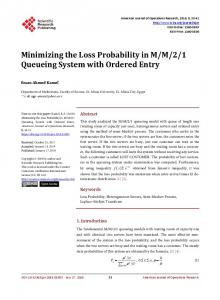
between incentives and efficiency: the optimal state-dependent policy, threshold allocation, performs better than the optimal state-independent policy, linear allocation. Additional comparisons among the policies can be made via some graphical examples. For each allocation policy, Figures 1 and 2 show the relationship between R and the equilibrium lead times with two examples: c(μi ) = 4μi and λ = 1; and c(μi ) = 4μ2i and λ = 1. We see from these figures that for a given price the buyer’s lead time can vary considerably. In all cases common-queue and proportional allocation with β = 1 perform poorly. Bell-Stidham allocation gives intermediate performance.

Balanced allocation performs reasonably well

when an equilibrium exists, but an equilibrium exists for a relatively limited range of prices (it never exists with linear capacity cost). Overall, threshold allocation is clearly the best, but linear allocation, especially given its simplicity, is a good second choice. The next lemma explores further the difference between linear and threshold allocation. Lemma 7 Define z(R) = Wsd (μt (R))/Wsi (μl (R)), where μt (R) and μl (R) are the equilibrium capacities under threshold and linear allocations respectively when the price is R. Recall that μt (R) = μl (R), i.e., for a fixed wholesale price threshold and linear allocation generate the same capacity. The ratio z(R) is concave and increasing from 1/2 to 1. The comparison between threshold and linear allocation is intuitive: if system utilization is quite high, because R is low, then threshold allocation has a single queue with a large number of jobs whereas linear allocation has two queues with a large number of jobs (i.e., threshold’s lead time is half of linear’s lead time); but if system utilization is quite low, because R is high, then jobs never wait with either allocation policy.

Although Lemma

7 indicates that linear allocation is significantly worse than threshold allocation when the buyer’s price is low, this result is somewhat misleading. Suppose now that the buyer is able to modify her price somewhat.

Let Rt be the price with threshold allocation and let Rl

be the price with linear allocation and choose these prices such that they lead to the same delivery lead time, Wsd (μt (Rt )) = Wsi (μl (Rl )). According to the next lemma, if Rt is either low or high, then there is a small price premium needed with linear allocation to achieve the same lead time. Lemma 8 Let ρ be the system’s utilization in equilibrium. Rl /Rt → 1 as either ρ → 1 or 13

ρ → 0. 3.3 Lead-time based allocation This section considers whether the buyer could do better (or at least as well) with an allocation policy based on the servers’ lead times rather than based on their capacities. In a lead-time based allocation, the buyer announces the demand share function λi in terms of servers’ lead time vector W = (W1 , W2 ) > 0, the servers submit their bids on lead times, demand shares are determined and each server i builds capacity μi (Wi , λi (W )) to fulfill its lead-time bid, where μi is a decreasing function of Wi . Assume λ1 (W ) − λ1 (Wε ) < μ1 (W1 , λ1 (W )) − μ1 (W1 + ε, λ1 (Wε ))

(7)

where Wε = (W1 + ε, W2 ) and ε > 0 : if server one promises a longer lead time then server one’s required capacity to achieve that lead time decreases more than server one’s demand allocation. The analogous assumption is taken for the other server as well. This assumption holds, for example, when each server operates an M/M/1 queue, in which case μi (Wi , λi (W )) = 1/Wi + λi (W ) .

(8)

Lead-time based allocation is analytically cleaner than capacity-based allocation because there is no issue with the stability of the queues: by definition, the buyer’s lead time is positive and finite for any strategic choice vector of the servers, whereas with capacity-based allocation the servers may fail to choose a sufficient capacity to yield a finite lead time for the buyer. However, according to the next lemma, analytical tractability can come with a price. Lemma 9 Consider any continuous lead-time allocation with λi decreasing in Wi . If (W1 , W2 ) is a Nash equilibrium with corresponding demand shares (λ1 , λ2 ) and μi (Wi , λi (W )) satisfies ˆ for all i, where μ ˆ is the solution to c0 (ˆ μ) = R. (If c(μ) is linear, (7) , then μi (Wi , λi (W )) ≤ μ

let μ ˆ = ∞).

Recall that μ ¯ is the servers’ maximum capacity (i.e., c(¯ μ) = Rλ/2) and the capacity achieved with linear or threshold allocation based on capacities. It is possible that the maximum achievable capacity with a lead-time based allocation policy, μ ˆ , is less than the maximum with a capacity based allocation policy, μ ¯ . We demonstrate this with two examples 14

in which the relationship between a server’s lead time and its capacity is given by (8), i.e., a state-independent allocation policy is implemented. First, suppose the capacity cost function √ is quadratic, c(μ) = aμ2 + bμ and a > 0. Then μ ¯>μ ˆ for all R ∈ (r1 , aλ + b2 + a2 λ), i.e., for sufficiently small R in the feasible range (R > r1 ) the buyer cannot design a continuous allocation policy based on the servers’ lead times that achieves the maximum capacity, μ ¯. Next suppose c(μ) = aμγ for a > 0 and γ > 1. In this case, ¡ Rλ ¢ γ1 1 µ ³ ´ 1 ¶ γ−1 μ ¯ r1 γ 2a =³ ´ 1 = γ , μ ˆ R R γ−1 γa

where recall that r1 = c(λ/2)/(λ/2) = a (λ/2)γ−1 . It follows that μ ¯>μ ˆ when R ∈ (r1 , r1 γ γ ),

i.e., lead-time based allocation is likely to be inferior to capacity based allocation as the buyer’s price is low and as the capacity cost function becomes more convex (γ increases). Despite the one-to-one relationship between a server’s lead time and the server’s capacity for a fixed allocation, lead-time based allocation may not be as effective as capacity-based allocation because lead-time based allocation has a self-restraining property that dampens competition among the servers: committing to a higher service level requires more investment than committing to a higher capacity. A similar result is obtained in Cachon and Zipkin (1999) in the context of inventory management in a serial supply chain with two independent firms: with non-strategic firms the optimal policy can be implemented as either a set of installation base stock policies or as a set of echelon base stock policies (briefly, these policies differ in what information they use) but with strategic firms these two approaches yield different equilibrium results.

4 Discussion This section discusses several modeling issues. Although we assume exponential processing times, some of our results extend to more general processing time distributions. As in Bell and Stidham (1983), suppose μ is the service rate and the service time S has first moment E(S) = 1/μ and second moment E(S 2 ) = bμ−2 . The variance is then (b − 1)μ−2 and the

coefficient of variation is constant, (b − 1)1/2 . For an M/G/1 queue with the above service

time distribution, the average lead time (duration in the system) is W (λ) =

1 bλ + . μ 2μ(μ − λ) 15

Balanced, linear, proportional, Bell-Stidham and threshold allocations readily extend to this general distribution because demand is allocated based only on the servers’ capacities and not on their lead times. However, the extension is not straightforward for common-queue because then the servers’ shares of demand are endogenously determined. Throughout our analysis we have assumed that each job is processed by only one server. In practice there are examples in which firms duplicate their orders across multiple suppliers or servers (see Armony and Plambeck 2005, Li 1992 and Yoffie 1990). If order duplication is feasible then it is ideal from the point of view of system efficiency: even if there is only one job in the system all servers are working at their full rate.

However, as we have

demonstrated, it is also important for an allocation policy to provide sufficient incentives for strategic servers to work hard. Zhang (2004) demonstrates that order duplication performs poorly on incentives, so poorly that its overall performance tends to be worse than linear allocation.

Hence, even if operating conditions are ideal for order duplication, a buyer

should avoid order duplication. We use demand allocation as the motivator to provide fast service, but other motivators may exist. For example, if the buyer has some control over the price, R, then raising the price, as we see in Figures 1 and 2, generates faster service (but with some allocation policies it also eliminates the existence of an equilibrium). The buyer could make a trade-off between the higher price paid and the faster service received.

Nevertheless, unless the price paid

is extremely high, there remains considerable variation in the performance of the allocation policies. Instead of allocating demand, the buyer could try to motivate faster service by posting a payment schedule that is contingent on the servers’ capacities or lead times. For example, suppose the buyer wants each server to build μ∗i > λ/2 capacity. This is achievable with the following price schedule, R(μi ), R00 (μi ) < 0,

R0 (μ∗i )(λ/2) = c0 (μ∗i )

and

R(μ∗i ) (λ/2) = c(μ∗i ) :

the first condition ensures a unique μi maximizes the server’s profit, the second condition ensures that μ∗i is optimal for the server and the third condition makes the server’s profit condition binding. It is also possible that the R(μi ) schedule could be implemented with a fixed price and late fees because then the late fees paid are contingent on the chosen capacity. (See Cachon and Zhang 2006 for a similar model with sole sourcing and late fees.) 16

Our

model does not address whether demand allocation is preferable to these or other contracting methods. However, we point out that these contracting methods require the buyer to posses significant bargaining power over the servers — the buyer must be able to control the pricing schedule used and its parameters, whereas demand allocation can be implemented by the buyer even if the buyer has little bargaining power. Therefore, because allocation policies are simple to implement and observed in practice, we suspect they are desirable vis-a-vis other techniques along at least some dimensions. Overall, additional research is needed to identify the situations in which demand allocation is the best option for the buyer. In our analysis we assume the suppliers have identical cost functions, which is reasonable in markets that have homogeneous technologies. This naturally leads to symmetric equilibria. With heterogenous cost functions, equilibrium analysis is more challenging. Zhang (2004) provides some initial results and finds that existence is less likely as costs become more heterogeneous: as one supplier gains a cost advantage it becomes necessary to dampen the competition among the suppliers to prevent one supplier from driving the other supplier out of the market, just like the problem we see when R is too high in the symmetric cost case. Hence, performance based allocation of demand appears to be most effective when suppliers have comparable costs. Our model assumes that each supplier only serves the buyer, as in the case when a supplier builds or reserves dedicated capacity for the buyer. In some cases each supplier may cater to multiple buyers, thereby creating two strategic decisions for each supplier: how much capacity to build and how to prioritize that capacity across buyers. Furthermore, there may be different prices for different priorities. The analysis of these systems is clearly beyond the scope of this research, but we again suspect that the buyer could use a smartly designed allocation policy to obtain higher priority from suppliers. We conduct our analysis in the context of a queuing system, but there are also situations that may be better modeled as an inventory system: e.g., each supplier could choose a base stock policy and the buyer is concerned with some dimension of the supplier’s delivery lead time distribution. While the specifics of the analysis would differ, we suspect that demand allocation would again be a useful tool for the buyer to motivate for better reliability among her suppliers. Our analysis is conducted exclusively in steady state. For example, we assume that the

17

buyer is able to infer each server’s capacity from the servers’ delivery times so that the correct demand share can be implemented. In practice the buyer would only obtain an estimate of each server’s capacity. The significance of sampling error on our results is an open question. Finally, we have implicitly assumed that the buyer is able to credibly commit to implement the chosen allocation policy. Without that ability, the buyer’s set of allocation policies to choose from is quite limited. For example, if the buyer must implement a state-independent policy, then only Bell-Stidham allocation is credible because it minimizes the buyer’s waiting time for any set of capacities chosen.

If the buyer implements a state-dependent policy,

then only threshold allocation is credible, but not necessarily the same threshold policy discussed in Section 3.2: again, the threshold policy must be chosen so as to minimize the buyer’s waiting time for any capacity vector.

Hence, the ability to credibly commit to an

allocation policy is important to the buyer. We note that this same issue occurs in many other settings. For example, in the supply chain contracting literature, many coordinating contracts are studied and observed that require commitments: a buy-back contract is an a priori commitment by a supplier to pay a retailer for units returned by the retailer after stochastic demand occurs even though the supplier has no ex post incentive to do so.

5 Conclusion In this paper two queuing servers strategically choose their capacities/processing rates in response to a buyer’s demand allocation policy.

The buyer’s objective is to design the

allocation policy to achieve the shortest possible average delivery time from the servers, either by motivating the servers to build more capacity or by ensuring that the available capacity is effectively utilized. We focus on allocation policies based on the servers’ capacities because we show that lead-time based allocation policies may not perform as well. Previous research suggests that there may exist a trade-off between incentives and efficiency: an allocation policy that efficiently utilizes the servers’ capacity may provide weak incentives for them to work quickly and an allocation policy with strong incentives to work quickly may not effectively utilize the servers’ capacity. We indeed demonstrate that there is considerable variation in the performance across allocation policies. Many allocation policies either provide absolutely no incentive for the servers to deliver quickly or provide too much competition among servers, thereby leading to unpredictable behavior. Even policies 18

that are optimal for the buyer with non-strategic and symmetric servers can perform poorly with strategic servers. However, we show that there need not be a trade-off between incentives and efficiency, i.e., there exists an allocation policy, threshold allocation, that induces the servers to work at their maximum rate and minimizes the buyer’s lead time given the resulting capacities. Unfortunately, threshold allocation is complex.

For example, its optimal parameters

cannot be determined in closed form. We offer linear allocation as an alternative. Linear allocation also induces the servers to work at the maximum possible rate, but linear allocation does not utilize the servers’ capacity as effectively as threshold allocation.

In particular,

because linear allocation allocates jobs immediately upon arrival and the assignment of jobs does not depend on the current state of the system (it is a state-independent allocation policy), linear allocation may allocate a job to a busy server while the other server is idle. Nevertheless, we show that linear and threshold allocations converge in performance at high utilizations, which suggests that linear allocation is attractive along many dimensions. To conclude, a buyer should not ignore demand allocation as a strategy to obtain faster service, especially given its simplicity: there is no need to negotiate new contract terms or pricing with the servers because demand allocation can be implemented by a buyer without the explicit consent of the servers. But creating competition among servers via their past performance requires some sophistication; a haphazard application of this strategy could have little impact.

Appendix Proof of Theorem 1. Server i’s profit function is π i (μi ) = Rλi − c(μi ). Let μ0i be defined such that μ0i > 0 and λi (μ0i ) = 0 or μ0i = 0. π i (μi ) is then concave and decreasing for μi ∈ [0, μ0i ].

Now differentiate π i , ⎛

∂π i (μi ) ⎜ = R ⎝1 − ∂μi

1/2 μi P 1/2 μj

⎞ ¢ 1/2 μj − λ μj ⎟ 0 − ³ ´2 ⎠ − c (μi ) 1/2 P 1/2 μj 2μi ¡P

and, for notational convenience, let B = μj − λ, 1/2

Rμj ∂ 2 π i (μi ) 1/2 −3/2 1/2 −1/2 = P 1/2 (μj Bμi + 3Bμ−1 − 1) − c00 (μi ). i − 3μj μi 2 3 ∂μi 4( μj ) 19

1/2 −3/2

Define f (μi ) = Bμj μi

1/2 −1/2

+ 3Bμ−1 i − 3μj μi

− 1.

If B ≤ 0, then π00i (μi ) ≤ 0 and

π i (μi ) is concave. Otherwise it can be shown that df/dμi = 0 has only one positive solution. Moreover, f → ∞ and df /dμi < 0 as μi → 0 and f < 0 as μi → ∞. Thus f decreases from the positive domain to the negative domain. Since c000 (μi ) ≥ 0, there exists a μ1i ≥ μ0i such

that πi (μi ) is concave and decreasing for μi ∈ [0, μ0i ], convex for μi ∈ [μ0i , μ1i ] and concave

for μ1i < μi . Because π i (0) = 0, it follows that any interior solution to server i’s first-order condition is a global optimum if at that solution profit is non-negative. The following equation provides the unique solution to the first-order conditions given the constraint μi = μj :

¶ µ ¶µ λ/2 R − c0 (μi ) = 0. 1+ 4 μi

(Because c(μi ) is convex, the left hand side is decreasing, so there is a unique solution.) The lower bound on R ensures that μbs > λ/2. The condition π i (μbs ) ≥ 0 ensures that μbs is indeed a global optimum for all servers.¤ Proof of Theorem 2: There are two significant complications to this analysis which prevent the use of standard existence and uniqueness results. (1) π i is not unimodal (if μ2 > λ, then π 1 is concave and decreasing for μ1 ∈ [0, μ2 − λ] and concave for μ1 > μ2 − λ, but not globally concave), which may create a discontinuity in the servers’ best reply functions. (2) π i is not differentiable at μi = λ − μj , which prevents the unconditional use of first-order conditions to determine the global maximizer of π i . Let’s first establish when {μb , μb } is a Nash equilibrium under the given conditions. The servers’ first-order conditions are satisfied when c0 (μb ) = R/2, which yields a finite lead time only if μb > λ/2, which simplifies to the first condition. But because μi = 0 can be optimal for a server, μb is an optimal response only if π i (μb , μb ) ≥ 0, i.e., if Rλ/2 ≥ c(μb ), which can be written as c0 (μb ) ≥ c(μb )/λ (the second condition). Now let’s rule out other equilibria. Suppose {μi , μj } is an equilibrium, μi ≥ μj . Several cases need to be considered. (i) μi ≥ λ + μj . If μj > 0, then server j earns a negative profit, so this is not an equilibrium. If μj = 0, then it must be that μi = λ. For server j we have πj (λ, μb ) = c0 (μb )μb − c(μb ) > 0, breaking the equilibrium. (ii) μi + μj < λ

which implies μj < λ/2. From server j’s first-order condition we get c0 (μj ) = R > 2c0 (λ/2),

which implies μj > λ/2 because c0 (·) is increasing. Hence, we have a contradiction, so no equilibrium. (iii) μi + μj = λ. For this to be optimal for both servers it must be that R ≤ 2c0 (μi ) and R ≤ 2c0 (μj ), which cannot both be satisfied because R > 2c0 (λ/2). (iv) 20

μi + μj > λ and μi < λ + μj . Now the only solution to the first-order conditions is {μb , μb }. To obtain an equilibrium with finite lead times, we need μi + μj > λ. Since μi ≥ λ + μj cannot be an equilibrium, there must be μi < λ + μj , which implies that {μb , μb } is the only solution to the first-order conditions. But {μb , μb } is not an equilibrium if c0 (μb ) < c(μb )/λ

and μb < λ/2 if R < r2 .¤ Proof of Theorem 3. (i) For Nash equilibrium we need to show that μl maximizes server i’s profit if the other server chooses μj = μl . The primary complication is due to the revenue term, Rλi (μ), in the profit function. Server i’s allocation is © ª λi (μ) = min (θμi /2 − θμl /2 + λ/2)+ , λ (µ µ ¶¶+ ) λ c0 (μl )μl = min θμi /2 − −1 ,λ 2 c(μl ) The second term is negative. So there exists some μ0i such that λi = 0 for all μi ≤ μ0i .

If

μi = μl then λi (μ) = λ/2. The condition R > r1 ensures that λ/2 < μl , so it follows that μ0i < μl . The server’s profit function is concave and decreasing for μi ≤ μ0i and concave and

continuous for μi > μ0i , although possibly not differentiable when λi (μ) = λ. For μi > μ0i , by construction of the parameters, π i is maximized with μi = μl and π i = 0 with μi = μl . Therefore, μl is optimal for server i.

Lead times are finite because μl > λ/2.

Next we

concentrate on uniqueness. Suppose μ is a Nash equilibrium of the capacity game. The proof first rules out asymmetric equilibrium with positive capacity for all servers and then equilibrium with μi = 0 for some i are ruled out. Suppose in some equilibrium μi > 0 for all i. (otherwise server i would make negative profit).

It must be then that λi > 0 for all i Thus, the first-order condition for each

server must be satisfied given n ˆ = 2, but that yields μi = μl for all i because the solution to each server’s first-order condition depends only on μi . Now suppose there exists a μi = 0 in equilibrium. All servers choosing μi = 0 cannot be an equilibrium because then one server could build a small amount of capacity and earn positive profit. If server 1 has the only positive capacity, then server 1 receives λ1 (μ) = λ as long as μ1 > 0; this cannot be an equilibrium because then server 1’s optimal capacity is some arbitrarily small capacity, which then allows the other server to build positive capacity and earn positive profit. (The condition μi > 0 for all i ≤ n ˆ in the allocation function is 21

critical to this result.) (ii) The proof is similar to (i), so it is omitted.¤ Proof of Theorem 4. For server i μβ−1 μβj ∂π i (μ) i = Rλβ P β − (2aμi + b), i = 1, 2. ∂μi ( j μj )2

Given R and β, simple algebra reveals that μi = μp is a symmetric solution to the first order conditions and it is the only solution. If each server chooses μp , then each server earns a zero profit. So it is an equilibrium if max πi = 0. Differentiate: i μβ−2 μβj h ∂ 2 π i (μ) i β β = Rλβ − (β + 1)μ (β − 1)μ ³ ´ j i − 2a. 3 ∂μ2i β β μi + μj

Note that β = 2¯ μc0 (¯ μ)/c(¯ μ) > 2. It can be shown (see Zhang 2004 for details) that π i is concave-convex-concave if μj = μp . Because π i = 0 and π 0i < 0 when μi = 0, it must be that max π i = 0. Therefore, μ1 = μ2 = μp is the unique Nash equilibrium of the capacity game.¤ Proof of Theorem 5. First demonstrate that μi = μp for all i is a unique Nash equilibrium when R > r2 . The first-order conditions must be satisfied: μj ∂πi (μ) = Rλ P − c0 (μi ) = 0, i = 1, 2. ∂μi ( j μj )2

(9)

The first-order conditions imply μi = μj , so the only solution must be μi = μp for all i. The condition R > r2 ensures the solution to the first-order conditions has μi > λ/2, which provides finite lead times. Now suppose R ≤ r2 and there is an equilibrium with finite lead times. If the lead times are finite then the first-order conditions (9) hold and only μi = μj satisfy them. Again, because lead times are finite, it must be that μi = μj > λ/2. Because each first-order condition is increasing in R, each first-order condition is maximized with R = r2 , in which case (9) can be written as c0 (λ/2)λ/(2μi ) − c0 (μi ) < 0 which means that μi = μj cannot be an equilibrium.¤ Proof of Lemma 6. See Kalai, Kamien, and Rubinovitch (1992).¤ Proof of Lemma 7. It is easy to determine that z(R) = μl / (μl + λ/2) and the results follow immediately given that μl ≥ λ/2.¤ Proof of Lemma 8. Each generates the maximum capacity, so c(μl ) = Rl (λ/2) and c(μt ) = 22

Rt (λ/2), which imply Rl /Rt = c(μl )/c(μt ). If waiting times are equivalent, then μ2t

μt 1 = 2 − (λ/2) μl − λ/2

which simplifies to μl /μt = 1 − ρ2 + ρ.¤ Proof of Lemma 9. Server i’s profit is

π i (W ) = λi (W )R − c(μi (Wi , λi (W ))). Let W be an equilibrium with μ1 (W1 , λ1 (W )) > μ ˆ . Define Wε = (W1 + ε, W2 ) and λε = λ1 (W )−λ1 (Wε ) : server 1 is allocated λε fewer units of demand because of the slower service provided to the buyer. Next we show that there exists an ε > 0 that would increase server 1’s profit, which leads to a contradiction. The difference between the profit functions can be written as π 1 (W ) − π1 (Wε ) = λε R − [c(μ1 (W1 , λ1 (W ))) − c(μ1 (W1 + ε, λ1 (Wε )))]. ˆ implies c0 (μ1 (W1 , λ1 (W ))) > R. Since λ1 is continuous, We know that μ1 (W1 , λ1 (W )) > μ for a sufficiently small ε, there is also c0 (μ1 (W1 + ε, λ1 (Wε ))) > R. By assumption, λε < μ1 (W1 , λ1 (W )) − μ1 (W1 + ε, λ1 (Wε )) , i.e., the required capacity decreases more than demand when the server provides worse service, we know that λε R < c(μ1 (W1 , λ1 (W ))) − c(μ1 (W1 + ε, λ1 (Wε ))) or π 1 (W ) − π 1 (Wε ) < 0. Therefore, there exists an ε that would increase server 1’s profit. As a result, W cannot be an equilibrium.¤

References Allon, G., A. Federgruen. 2003. Competition in service industries. forthcoming Operations Research. Anton, J.J., D.A. Yao. 1989. Split awards, procurement, and innovation. Rand Journal of Economics. 20(4) 528-552. 23

–, –. 1992. Coordination in split award auctions. The Quarterly Journal of Economics. Anupindi, R., R. Akella. 1993. Diversification under supply uncertainty. Mgmt Sci. 39(8) 944-963. Armony, M., E. Plambeck. 2005. The impact of duplicate orders on demand estimation and capacity investment. Mgmt Sci. 51(10):1505-1518. Bell, C., S. Stidham. 1983. Individual versus Social Optimization in the Allocation of Customers to Alternative Servers. Mgmt Sci. 29. 831-839. Benjaafar, S., E. Elahi, K. Donohue. 2004. Outsourcing via service quality competition. forthcoming Management Science. Bernstein, F., G. DeCroix. 2004. Decentralized pricing and capacity decisions in a multi-tier system with modular assembly. Mgmt Sci. 50. 1293-1308. –, F. de Vericourt. 2005. Competition for procurement contracts with service guarantees. forthcoming Operations Research. Bonser, J.S., S.D. Wu. 2001. Procurement planning to maintain both short-term and adaptiveness and long-term perspective. Mgmt Sci. 47(6) 769-786. Cachon G.P., P.T. Harker. 2002. Competition and outsourcing with scale economies. Mgmt Sci. 48(10) 1314-1333. –, M.A. Lariviere. 1999a. Capacity allocation using past sales: when to turn and earn. Mgmt Sci. 45(5) 685-703. –, –. 1999b. Capacity choice and allocation: strategic behavior and supply chain performance. Mgmt Sci. 45(8) 1091-1108. –, –. 1999c. An equilibrium analysis of linear, proportional and uniform allocation of scarce capacity. IIE Transactions. 31(9) 835-850. Cachon, G.P., F. Zhang. 2006. Procuring fast delivery: sole-sourcing with information asymmetry. Mgmt Sci. 52(6). 881-96. Cachon, G.P., P.H. Zipkin. 1999. Competitive and cooperative inventory policies in a twostage supply chain. Mgmt Sci. 45(7) 936-953. Chayet, S., W. Hopp. 2002. Lead time competition under uncertainty. Working paper, Northwestern University.

24

Chen, J., D.D. Yao, S. Zheng. 2001. Optimal replenishment and rework with multiple unreliable supply sources. Oper. Res. 49(3) 430-443. Christ, D., B. Avi-Itzhak. 2002. Strategic equilibrium for a pair of competing servers with convex cost and balking. Mgmt Sci. 48(6): 813-820. Deshpande, V., L. Schwarz. 2002. Optimal capacity choice and allocation in decentralized supply chains. Working paper, Purdue University. Elmaghraby, W.J. 2000. Supply contract competition and sourcing strategies. MSOM. 2(4) 350-371. Farlow, D., G. Schmidt, A. Tsay. 1996. Supplier management at Sun Microsystems (A). Stanford Business School Case. Gallien, J., L.M. Wein. 2005. A smart market for industrial procurement with capacity constraints. Management Science. 51(1). 76-91. Gilbert, S.M., Z.K. Weng. 1998. Incentive effects favor nonconsolidating queues in a service system: the principle-agent perspective. Mgmt Sci. 44(12) 1662-1669. Ha, A.Y., L. Li, S.-M. Ng. 2003. Price and delivery logistics competition in a supply chain. Mgmt Sci. 49(9) 1139-1153. Hassin, R., M. Haviv. 2003. To Queue or Not to Queue: Equilibrium Behavior in Queueing Systems. Kluwer Academic Publishers. Kalai, E., M.I. Kamien, M. Rubinovitch. 1992. Optimal service speeds in a competitive environment. Mgmt Sci. 38(8) 1154-1163. Koole, G. 1995. A simple proof of the optimality of a threshold policy in a two-server queuing system. Systems and Control Letters. 26. 301-303. Lederer, P.J., L. Li. 1997. Pricing, production, scheduling, and delivery time competition. Oper. Res. 45(3) 407-420. Li, C.-L., P. Kouvelis. 1999. Flexible and risk-sharing supply contracts under price uncertainty. Mgmt Sci. 45(10) 1378-1398. Li, L. 1992. The role of inventory in delivery-time competition. Mgmt Sci. 38(2) 182-197. Lin, W.P. R. Kumar. 1984. Optimal control of a queuing system with two heterogeneous servers. IEEE Transactions Automat. Control. 29. 696-703.

25

Martinez de Albeniz, V., D. Simichi-Levi. 2003. Competition in the supply option market. Working paper, MIT. Minner, S. 2003. Multiple-server inventory models in supply chain management: a review. International Journal of Production Economics. 81-82 265-279. Nagarajan, M., Y. Bassok. 2003. A bargaining framework in supply chains. Working paper, USC. Naor, P. 1969. On the regulation of queue size by levying tolls. Econometrica. 37. 15-24. Pyke, D., E. Johnson. 2003. Sourcing strategies and server relationships: alliances vs. eprocurement. Forthcoming in The Practice of Supply Chain Management, eds. C. Billington, H. Lee, J. Neale, T. Harrison. Kluwer Publishing. Rubinovitch, M. 1985a. The slow server problem. J. of Applied Prob.. 22 205-213. Rubinovitch, M. 1985b. The slow server problem: a queue with stalling. J. of Applied Prob.. 22 879-892. Sedarage, D., O. Fujiwara, H.T. Luong. 1999. Determining optimal order splitting and reorder level for N-server inventory systems. Euro. J. of Oper. Res. 116 389-404. Seshadri, S. 1995. Bidding for contests. Mgmt Sci. 41(4) 561-576. –, K. Chatterjee, G.L. Lilien. 1991. Multiple source procurement competitions. Marketing Sci. 10(3) 246-263. So, K.C. 2000. Price and time competition for service delivery. MSOM. 2(4) 392-409. Talluri, S. 2002. A buyer-seller game model for selection and negotiation of purchasing bids. Euro. J. of Oper Res. 143(1) 171-180. Walgrand, J. 1984. A note on “Optimal control of a queuing system with two heterogeneous servers”. Systems Control Letters. 4. 131-134. Wang, Y., Y. Gerchak. 2003. Capacity games in assembly systems with uncertain demand. MSOM, 5(3) 252-267. Yoffie, D.B. 1990. The global semiconductor industry, 1987. In International Trade and Competition: Cases and Notes in Strategy and Management. D.B. Yoffie (ed). McGrawHill. New York. 389-413. Zhang, F. 2004. Coordination of lead times in supply chains. Dissertation, University of

26

Pennsylvania.

27

4.0 3.5

Lead time

3.0 2.5 2.0 t

l

6

8

bs

p

c

1.5 1.0 0.5 0.0 4

10

12

14

16

18

20

22

24

26

28

30

R

Figure 1: The lead time received by the buyer as a function of the price paid, R, and the allocation policy with capacity cost c( μi ) = 4μi and λ = 1. t = threshold policy, l = linear allocation, bs = Bell-Stidham, c = common queue, p = proportional allocation with β = 1. (Balanced allocation is not included because an equilibrium does not exist in this setting.)

4.0 3.5 3.0

Lead time

2.5 2.0

t

l

b

bs

c

p

1.5 1.0 0.5 0.0 2

4

6

8 10 12 14 16 18 20 22 24 26 28 30 32 34 36 38 40 R

Figure 2: The lead time received by the buyer as a function of the price paid, R, and the allocation policy with capacity cost c( μi ) = 4μi 2 and λ = 1. t = threshold policy, l = linear allocation, b = balanced allocation, bs = Bell-Stidham, c = common queue, p = proportional allocation with β = 1.