OCEAN MODELING IN ISOPYCNIC COORDINATES. RAINER BLECK. Rosenstiel School of Marine and Atmospheric Science. University of Miami.
OCEAN MODELING IN ISOPYCNIC COORDINATES RAINER BLECK Rosenstiel School of Marine and Atmospheric Science University of Miami 4600 Rickenbacker Causeway Miami, Florida 33149, USA D r a f t { May 1, 1998
1. Introduction Electronic computers were made available to civilian researchers in the late 1940s, shortly after World War II. Numerical Weather Prediction { at that time the repetitive solution of a 2-dimensional elliptic partial di�erential equation describing the evolution of the height of a mid-tropospheric isobaric surface { was among the rst mathematical problems tackled with that new technology. A decade or so later, when computers were fast enough to allow adding a third (vertical) dimension to NWP models, mathematical complexities created by variable terrain height led to the development of a special vertical coordinate � = p=psurface which removed mountain-induced \bumps" from the computational domain [14] . The � coordinate quickly became the coordinate of choice in NWP models, but the community eventually realized that the search for the perfect vertical model coordinate was far from over. One can say that it is still going on today. Accuracy and stability problems created by the vertical advection terms in the prognostic equations formulated in z , p, or � coordinates led to early experimentation with models formulated so as to minimize the role of these terms [21]. While isentropic (�) coordinate models achieve this goal at least under adiabatic ow conditions, such models never became popular because of concerns about numerical stability at the lower boundary whose location in � space is irregular even in the absence of mountains and varies with time. Advances in hybrid coordinate technology have laid these problems to rest today, allowing isentropic NWP models | speci cally, mixed �-� coordinate models | nally to achieve operational status.
2
RAINER BLECK
Modeling the oceanic circulation has lagged behind NWP for reasons having to do with insu�cient economic incentives, lack of observations, and the combination of long time scales with the small size of oceanic eddies which makes ocean modeling a more resource-intensive task. Thus, only a few large research institutions were able to commit the resources needed for developing ocean models. Perhaps inevitably, the ocean model \gene pool" remained sparse over the years, and instances of model \inbreeding" were common. Only today, as more and more academic researchers gain access to large computers, do we see the diversity in ocean modeling reminiscent of the NWP culture of the 1960s and '70s. Models using density or, more precisely, potential density as vertical coordinate are one example of the growing ocean model diversity. Development of such models has been driven by the community's increasing awareness of numerical errors inherent in z and � coordinate models | errors having to do with the physically inappropriate (though mathematically correct) split of transport and di�usion processes into vertical and horizontal components. Isopycnic (constant potential density) models suppress such errors to a large extent by, essentially, switching the role of density and depth as dependent and independent variables. Not only does this reduce inconsistencies between vertical and horizontal transport terms, but it allows one to hide truncation errors associated with the remaining horizontal transport terms behind the \smoke screen" of isopycnic mixing. The purpose of this article is to review the numerical tools needed for solving equations in which depth is a dependent variable and potential density an independent variable, and to present results illustrating the unique diagnostic capabilities of such models.
2. Dynamic Equations Primitive-equation models using potential density as vertical coordinate [13] [6] typically contain 3 or 4 prognostic equations { one equation for the horizontal velocity vector, a mass continuity or layer thickness tendency equation, and either one or two conservation equations for buoyancy-related variables (density, salt, temperature). Since not all coordinate layers in an isopycnic model are necessarily constant-density layers (prime example: the surface mixed layer discussed below), the equations will be written here for a nondescript, generalized vertical coordinate s [3]. Density � and its inverse, speci c volume �, represent in-situ conditions, but it will be shown later that the equations remain valid if these variables are corrected for compressibility e�ects, i.e., if they are interpreted as potential density and its inverse.
3
ISOPYCNIC MODELING
The equations, in the order mentioned above, are � @p � @ v 2 v @v + rs 2 + (� + f )k � v + s_ @s @p + r� M @ts � � @p @ � � @p �?1 = ?g @p + @s rs � � @s rs v � @p � @ � @p � @ � @p � + r � + @s s_ @s = 0 s v @ts @s @s
(1) (2)
� @p � @ � @p � � @p � @ � @p � T + rs � v T + s_ T = rs � � rsT + HT (3) @ts @s @s @s @s @s
Here, v = (u; v) is the horizontal velocity vector, p is pressure, T represents any one of the model's thermodynamic variables (temperature, salinity, buoyancy), � = @v=@xs ? @u=@ys is the relative vorticity, M � � + p� is the Montgomery potential, � � gz is the geopotential, f is the Coriolis parameter, k is the vertical unit vector, � is the isopycnic eddy viscosity, and � is the wind- and/or bottom-drag induced shear stress vector. HT represents the sum of the diabatic source terms acting on T . Subscripts indicate the variable held constant during partial di�erentiation. Distances in x; y direction (as well as their time derivatives x_ � u and y_ � v) are measured in the projection onto a horizontal plane, a convention which eliminates metric terms related to the slope of the s surface. Isopycnic models are typically formulated as layer models, meaning that a number of prognostic variables are not carried on coordinate surfaces but represent conditions averaged over individual layers; they must therefore be advanced in time using layer-averaged equations. Averaging over a layer bounded by two surfaces stop ; sbot entails multiplying the equation in question by @p=@s, integration over the interval �s = sbot ? stop , and division by �p = p(sbot ) ? p(stop ). The ocean surface, the bottom of the mixed layer, the sea oor, and all isopycnic layer interfaces are considered s surfaces here. The layer-averaged continuity equation (2) becomes a prognostic equation for the layer weight per unit area or pressure thickness �p: � @p � � @p � @ � p + rs � (v�p) + s_ ? s_ = 0: (4) @t @s @s s
bot
top
The expression (s@p=@s _ ) represents the vertical mass ux { taken to be positive if in +p or downward direction { across an s surface.
4
RAINER BLECK
Layer-averaging the momentum equation (1) changes the shear stress term ( rst term on the right) into g �p (� top ? � bot )
while the lateral momentum mixing term integrates to (�p)?1 rs � (� �p rsv): (5) All other terms in (1) retain their formal appearance during the averaging operation. Wind-induced stress is assumed to be zero at the bottom of the uppermost coodinate layer, which therefore must not be allowed to become shallower than the Ekman layer. Bottom stress is partitioned among coordinate layers in accordance with the assumption that it linearly decreases from -�cD jvjv at the sea oor to zero over a prescribed depth interval of order 10 m. v in this formula is the velocity vector averaged over those 10 m. The layer-integrated form of (3) is � @p � � @p � @ ? s_ T = rs � (� �p rsT ) + HT : T �p + rs � (vT �p) + s_ T @t @s bot @s top (6) The above prognostic equations are complemented by diagnostic equations including the hydrostatic equation
@M = p; (7) @� an equation of state linking T; S; p to �, and an equation governing cabbeling in models where both T and S are treated as prognostic thermodynamic variables. The interlayer mass ux (s@p=@s _ ) must also be be prescribed. At
the bottom of the surface mixed layer, this ux is the result of mixed-layer entrainment and detrainment processes and can be quite large, while at interior interfaces it re ects diapycnal mixing processes which typically are weak. The quickest way to demonstrate the connection between diapycnal mixing and interlayer mass exchange is to start from the di�usion equation in z coordinates, � @� � @F = @z ; @t z
where F is the di�usive ux of the variable � (for example, ?K@�=@z ), and to use the identity (@a=@b)c (@b=@c)a (@c=@a)b = ?1 to exchange dependent and independent variables. The nal result of these manipulations is � @z � @F : = ? @t @� �
ISOPYCNIC MODELING
5
The derivative (@z=@t)� in this equation expresses the rate at which a divergent or convergent ux F causes the surface � = const: to migrate vertically through the uid, i.e., the rate at which mass is transferred from one side of the � surface to the other. Diapycnal mixing can easily be suppressed in isopycnic models, both physically and numerically, by setting s@p=@s _ = 0. Coordinate layers remain materially insulated from each other in this case.
3. Numerical Issues Selecting a set of di�erential equations is an essential rst step in building a circulation model, but before the equations can be solved on a computer, they must be converted into a set of algebraic equations. This conversion process is the essence of \numerical modeling", a eld that has seen remarkable growth since the rst failed attempts at NWP early in this century [18]. Certain tools needed for numerically solving uid dynamics equations in (x; y; �) space were not available in the 1960s when ocean models were rst conceived; it was therefore appropriate to design those rst-generation circulation models around a geometric vertical coordinate. In this section, the main tools employed in solving the primitive equations in (x; y; �) space will be discussed. 3.1. LAYER OUTCROPPING An isopycnic model may be viewed as a stack of shallow-water models in which the individual 2-dimensional submodels interact primarily through hydrostatically transmitted pressure forces. Since the top-to-bottom density range in a water column varies with geographic location, not all isopycnic coordinate layers can be expected to exist everywhere in the computational domain. Hence, provisions must be made for layers in the model to \vanish", i.e., to reach zero thickness. This is what is referred to as the layer outcropping problem. A closely related problem is that of coordinate layers intersecting the sea oor. Methods for numerically solving the layer thickness equation (4) in a way that allows the limit �p = 0 to be reached { but not overshot { became available in the late 1960s [27]. These methods belong to a by now large and diverse group of transport schemes designed to preserve the positive-de niteness of the transported variable [22]. Typically, they are 2step schemes where the variable in question (layer thickness �p in our case) is rst advected by a simple forward-upstream scheme that is guaranteed to maintain positive-de niteness of the advected eld. The positive-upstream step is followed by an antidi�usive step, so named because it is designed
6
RAINER BLECK
to counteract the di�usive e�ects of the rst step without jeopardizing the positive-de niteness and, optionally, the monotonicity of the transported eld. (Preserving monotonicity is akin to not permitting new maxima or minima to appear.) It is of interest to note that Oberhuber [13] solves the outcropping problem in his OPYC model by keeping track of the lateral extent of each coordinate layer. In the case of the Miami Isopycnic Coordinate Ocean Model (MICOM), the decision to use one of the general-purpose transport schemes was made because of the ease with which they can be vectorized and parallelized. 3.2. TOPOGRAPHIC INTERACTIONS Swift meridional currents in the ocean are generally found near basin boundaries where sidewall drag helps close the potential vorticity budget. The credibility of an ocean model therefore depends strongly on its ability to correctly portray the interaction between boundary currents and topography. One important issue is the computation of the horizontal pressure gradient normal to the boundary. The method used in MICOM for evaluating the pressure gradient near topographic obstacles dates back to [4] and is outlined more fully in [5]. The guiding design principle is to assure that a resting ocean with horizontal layer interfaces remains at rest. This is achieved by switching to noncentered di�erencing if one of the two M values in the centered nite-di�erence formula for @M=@x or @M=@y in (1) is associated with a massless grid cell on the sea oor. (If both M values are in massless grid cells, there is no need to compute a pressure force.) It is fair to say that the above method has withstood the test of time and that steep topography is a \non-problem" in MICOM. 3.3. ISOPYCNIC TRANSPORT EQUATIONS The equation dT=dt = 0 expressing conservation of a variable T in x; y; z space can be stated either in ux form, @u�T @�T = ? @t @x
or in advective form,
@T = ?u @T @t @x
@w�T ? @v�T ? ; @y @z
(8)
? v @T ? w @T : @y @z
(9)
The two forms do not a priori lead to the same result if solved numerically. However, the near-constancy of � in the ocean blurs the distinction between
ISOPYCNIC MODELING
7
them to such an extent that it is possible to advance T in z coordinate models using the simple advective form (9) without jeopardizing global conservation of T . The conservation equation analogous to (8) governing transport of T in isopycnic layer models is @ @ @ ( T �p) = ? (uT �p) ? (vT �p) @t @x @y
(10)
where we have omitted the diapycnal transport component for simplicity's sake. In this case, �p cannot be treated as quasi-constant the way � can be treated in the z coordinate version of the same conservation law. Rather, �p must be allowed to vary signi cantly from one location and one time step to the next. This precludes the use of a simple advective equation analogous to (9) in isopycnic models. Furthermore, after T �p has been advanced over one time step and is being divided by �p to obtain the new T value, provisions must be in place for the case where �p has dropped to zero during that time step. Experience has shown that the strong temporal and spatial variability of the �p eld requires use of positive-de nite, and preferably monotonicitypreserving, transport schemes not only for �p but for thermodynamic variables as well. Unfortunately, the extra computer time needed in isopycnic models to advect thermodynamic variables, tracers, etc., by an elaborate 2-step scheme cancels the potential speed advantage that isopycnic models have over z coordinate models due to the fact that they can resolve baroclinic structures (fronts etc.) with considerably fewer grid levels than z coordinate models. In fact, the computational burden associated with solving (10) makes it advisable to treat only one thermodynamic variable { salinity { as prognostic variable in isopycnic layers while inferring the other { potential temperature { from the salinity and potential density. While explicit transport and di�usion of two thermodynamic variables in � coordinates seems redundant, it does permit modeling of cabbeling e�ects and helps guarantee global conservation of both T and S in the model. 3.4. BUOYANCY FORCING Isopycnic models were initially developed for simulating the wind-driven circulation. While mechanically driven isopycnic models seem to be devoid of a thermodynamic component, the conservation equation for potential density is, in fact, included in the set of model equations in the form of a statement prohibiting mass exchange between coordinate layers. The absence of a transport/di�usion component across layer interfaces under adiabatic
ow conditions was already mentioned as the main reason for developing isentropic NWP models and isopycnic ocean models.
8
RAINER BLECK
Conceptual problems arise in isopycnic models if the forces driving the circulation include buoyancy uxes, not only because buoyancy is an independent variable in these models, but also because discretization of the governing equations in the vertical implies that only a nite number of discrete density values are permitted in the model. The fact that buoyancy is an independent variable requires that another variable must be found that can properly respond to extraneously imposed buoyancy changes. This variable is the isopycnic layer thickness. Speci cally, buoyancy gains at the surface must be translated in isopycnic models into mass transfer from heavier to lighter layers; in case of surface buoyancy loss the direction of mass transfer is in the other direction. Di�culties created by the discrete density structure can be addressed in isopycnic models by allowing density in the uppermost model layer (the surface mixed layer) to vary continuously in x, y, and t. Adding this extra nonisopycnic layer clearly does not remove the physical incompatibility between the continously varying sea surface density eld and the discrete density structure in the model interior. Rather, the \clash" between the two representations is only shifted from the sea surface to the bottom of the nonisopycnic layer where vertical mass exchange must be allowed to take place in a way that mimics the physics of mixed-layer entrainment and detrainment. While there are no numerical di�culties in entraining water from constant-density layers into a nonisopycnic layer, the opposite process of mixedlayer detrainment clearly is problematic because water cannot simply be transferred out of the mixed layer unless its density matches that of an interior isopycnic layer. A sensible way to deal with the detrainment problem is to divide the uppermost model layer conceptually into a \physical" and a \fossil" mixed layer (the fossil mixed layer consisting of water that at one time was, but no longer is, in the physical mixed layer and is now awaiting transfer to an interior isopycnic layer). During detrainment, which occurs when the ocean is warmed or freshened from above, the fossil mixed layer grows at the expense of the physical mixed layer. The fossil mixed layer is now conceptually divided into two sublayers, and buoyancy is exchanged between the two sublayers until the upper sublayer assumes the buoyancy of the physical mixed layer while the lower sublayer assumes the buoyancy of an interior coordinate layer. (The unknown in this problem is the depth of the interface separating the two sublayers.) This vertical redistribution of buoyancy allows one to combine the upper sublayer with the physical mixed layer into a single, vertically homogeneous coordinate layer, while the water from the lower sublayer can be detrained into the targeted isopycnic layer. Thus, during mixed-layer
ISOPYCNIC MODELING
9
detrainment episodes the uppermost model layer is usually deeper than the physical mixed layer. 3.5. COMPRESSIBILITY OF SEA WATER Eddy-induced mixing in a strati ed uid preferentially takes place along surfaces on which laterally displaced uid particles experience no restoring buoyancy force. These surfaces are referred to as neutral [15] [11]. The ocean is a near-incompressible, weakly strati ed medium. If it were totally incompressible, constant-density and neutral surfaces would coincide. With compressibility being nonzero, neutral surfaces in the real ocean coincide with potential density surfaces referenced to a nearby pressure level. Ocean models whose coordinate surfaces are neutral can be expected to simulate eddy-induced mixing far more accurately than models operating on a rigid lattice of grid points. (This has to do with the component represenation of the mixing process mentioned in the Introduction.) While isopycnic models come close to this ideal, especially if \isopycnic" is understood to mean constant potential density, the physical properties of sea water are such that perfect alignment of coordinate surfaces with neutral surfaces is di�cult to achieve near water mass boundaries at depths di�ering from the chosen reference pressure. This issue will be discussed further in the section on presently unsolved problems. Accurate simulation of mixing processes is only one concern in climateoriented ocean modeling; another one is accurate representation of circulations driven by temperature and salinity contrasts imposed on the ocean by the atmosphere. The term in the dynamic equations controlling the onset and maintenance of buoyancy-driven circulations is the curl of the 3-dimensional pressure acceleration, rH � �rp = (r�) � (rp); this term spawns the familiar solenoidal term �dp in Bjerknes' Circulation Theorem. We see from it that only isobaric density contrasts are capable of driving circulations; in other words, density contrasts resulting from the weight of the overlying uid alone are dynamically passive. The practice of de ning coordinate layers in isopycnic models in terms of potential density provides a convenient mechanism for eliminating dynamically passive density variations from the dynamic equations. This point deserves a closer look. As long as the adiabatic compressibility coe�cient � = �?1 (@�=@p)adiab is constant, or at most a function of pressure, it can be shown that rp� = rp�pot (11) � � pot
where �pot is the inverse potential density and rp is the 2-dimensional gradient operator on an isobaric surface. With � di�ering from �pot by no
10
RAINER BLECK
more than 2% in the world ocean, we conclude that
rp� � rp�pot : Integration of this equation over p (a step equivalent to integrating the thermal wind equation) yields
rp� � rp��
(12)
where �� is a geopotential-like function obtained by substituting �pot for � on the right-hand side of the hydrostatic equation @�=@p = ?�. Since rp� equals the horizontal pressure gradient, we conclude that circulationinducing pressure forces resulting from spatial variations in the � eld can be computed, with at most a 2% error, from the knowledge of the �pot eld alone. This obviates the need to carry in situ density as a variable in isopycnic models. Unfortunately, sea water compressibility is not only a function of pressure, but also of temperature: water near the freezing point is more compressible than water a few degrees warmer. Since water density near the freezing point is mainly a function of salinity, we can also state: given two low-temperature water parcels of equal density but di�erent salt content, the less saline parcel is more compressible. This so-called thermobaric e�ect invalidates the assumptions on which (11) and subsequent conclusions are based, and there are in fact situations where thermobaricity drives circulations that cannot be captured by the standard set of isopycnic model equations. A solution recently proposed by [19], and successfully tested by [24], consists of splitting the compressibility coe�cient � into a p- and a T -dependent part and using only the former in determining the potential density of a water parcel. The new variable, named �� to distinguish it from the genuine �pot , allows us to replace (11) by rp� = rp�� � �� and retain (12) with the stipulation that �� is obtained by integrating a hydrostatic equation of the form @�� =@p = ?�� . The variable �� { the inverse of what in [19] is called \virtual" potential density �� { does not appear to obey any conservation law. In particular, surfaces of constant �� are not material, even under adiabatic conditions. The strategy followed in MICOM is therefore to retain the variable �pot , which is material under adiabatic conditions, as vertical coordinate, and to treat �� as an (x; y; �pot ; t)-dependent diagnostic variable.
ISOPYCNIC MODELING
11
3.6. DEEP CONVECTION
Isopycnic coordinate models turn into single-layer shallow-water models in regions where the water column is homogeneous. Loss of strati cation can either be caused by a divergent surface ow eld (which brings dense subsurface water to the surface) or by buoyancy loss to the atmosphere. In the real ocean, surface buoyancy loss triggers convection which hydrostatic models, the model class to which MICOM belongs, are unable to simulate correctly. Parameterization of buoyant convection is therefore an important issue in such models. Compared to the level of sophistication reached by convective parameterization schemes in modern NWP models, the so-called convective adjustment scheme used in today's hydrostatic ocean models is embarassingly simple. In isopycnic models, convective adjustment is implemented by checking in each water column whether an isopycnic layer of nonzero thickness exists whose density is less than that of the surface mixed layer. If this is the case, the mass from the layer in question is transferred to the mixed layer and the thickness of the donor layer is set to zero.
4. Solved and Presently Unsolved Problems Isopycnic ocean models of the type represented by MICOM and Oberhuber's OPYC model have been in service for several years now, and their general utility is no longer being questioned. The question that remains in many people's mind, however, is whether these models are in an overall sense superior to the rst-generation xed-grid models. Some of the issues that in the past have delayed model acceptance, and some that still do because they either have not yet been tackled or are actually unsolvable, will be discussed in this section. 4.1. LAYER OUTCROPPING
The layer outcropping problem, although it was laid to rest 10 or 15 years ago, still is regarded by many as the number one problem in isopycnic modeling. \Laying to rest" in this case does not mean that layer outcropping as such has been eliminated as a physical or numerical phenomenon. It means that numerical methods have been developed { for example, the massless layer approach [4] [25] { which are su�ciently robust to eliminate layer outcropping as a hindrance to further advances in isopycnic modeling. One aspect still in need of attention is the numerical treatment of the wedge of unbounded potential vorticity along outcrop lines caused by vanishing layer thickness [1].
12
RAINER BLECK
4.2. SURFACE PROCESSES IN A DISCRETIZED DENSITY ENVIRONMENT The discrete density structure in isopycnic models and its impact on mixed layer physics parameterization is a more pressing concern. The treatment of sea surface density �surf most consistent with the discrete layer paradigm would be to set �surf at every point x; y to the value associated with the uppermost mass-containing (outcropping) coordinate layer. When buoyancy forcing was introduced into MICOM, the disadvantages of having to formulate air-sea interaction processes on the basis of a piecewise constant �surf eld were considered severe, and the strategy of allowing the uppermost coordinate layer to have characteristics di�erent from those of the remaining layers { namely, to be nonisopycnic { was regarded as the lesser evil. As outlined earlier, buoyancy uxes across the air-sea interface in an isopycnic model must be translated into mass uxes { speci cally, mass
uxes through the bottom of the mixed layer. It was also discussed that in the present MICOM implementation the numerical mismatch between the nonisopycnic surface mixed layer and the isopycnic model layers can lead to temporary di�erences between the physical mixed-layer depth and the thickness of the uppermost model layer. If maintaining the identity between mixed-layer depth and uppermost layer thickness is considered important in a particular model application, then this mismatch, caused by the presence of \fossil" mixed-layer water in the top coordinate layer, becomes a model error. However, it is a true truncation error in the sense that it can be reduced to any degree desired by increasing vertical model resolution, i.e., by adding more layers. Nevertheless, not all modelers accustomed to truncation errors in z space nd it easy to tolerate this particular shortcoming. As a rst step toward improving mixed-layer physics in MICOM, it is planned to split the uppermost model layer consisting of the surface mixed layer and the underlying \fossil" mixed layer into two separate layers. To discourage unlimited buildup of the so-de ned fossil layer, the detrainment mechanism described earlier for the mixed layer should in this case be applied to the fossil layer. The above procedure does not represent a radical departure from the presently used Kraus-Turner [8] mixed-layer parameterization scheme. More elaborate schemes are available today and are expected to eventually nd their way into isopycnic models. 4.3. THERMOBARICITY Another area of concern is the treatment of the equation of state, and in particular the traditional practice of regarding the ocean in isopycnic
ISOPYCNIC MODELING
13
models as strati ed but incompressible. The view that isopycnic models treat the ocean as incompressible is actually not quite correct. As pointed out earlier, density changes caused by the weight of the overlying uid are dynamically passive. The resulting dynamic equivalence of in situ and potential density makes it appear as though the model equations are founded on an incompressibility assumption when, in fact, they are not. As discussed earlier, a satisfactory method now exists for incorporating thermobaric e�ects into the modeling of buoyancy-driven circulations. However, thermobaricity has other consequences, some of which possibly belong to the class of principally unsolvable problems in isopycnic modeling. The consequences referred to have to do with the multivalued nature of �pot (z ), that is, with coordinate folding. Outside convective regions, the ocean is stably strati ed, but to verify this one must measure the static stability in terms of potential density referenced to the \local mean" pressure. The variable �pot de ning the layer structure in isopycnic models, on the other hand, must be based on a \global" choice of reference pressure. The work of Pingree [15], Reid [17], and others contains numerous examples of how spatial salinity variations combined with a nonlocal reference pressure can lead to grossly erroneous estimates of the �pot di�erence between pairs of water parcels, including the appearance of static instability when, in fact, the column is stably strati ed. Note the emphasis here on salinity variations, which seemingly contradicts the notion that adiabatic compressiblity � depends only on T and p. To resolve the contradiction, one must realize that in an isopycnic reference frame T variations are tightly coupled to S variations. There is no single reference pressure value that would not create coordinate folding at least somewhere in the world ocean. The best one can do therefore is to nd a reference pressure that minimizes instances of multivaluedness in �pot (z ) in the model initial conditions, and to smear out the vertical �pot distribution in the remaining overturning regions. The neutrally strati ed patches of water hereby created will, of course, not be intersected by coordinate surfaces and thus will su�er from poor vertical resolution unless one chooses to ll them with coordinate surfaces de ned in a di�erent manner (hybrid coordinates). Short of causing coordinate overturning, an inappropriately chosen reference pressure will also ruin the alignment of coordinate surfaces with neutral surfaces in regions marked by pronounced salinity variations. The adverse impact of this on the accuracy of mixing simulations could in principle be lessened by borrowing a tool originally designed for z coordinate models, namely, the rotation of the main axes of the mixing tensor [16].
14
RAINER BLECK
4.4. CONVECTION
The convective adjustment scheme described earlier is attractive in its simplicity but has the disadvantage of causing temporal discontinuities in layer thickness in the model. In the long run, convective adjustment schemes in isopycnic models should therefore be replaced by schemes that parameterize the sinking of dense plumes from the mixed layer to the interior layers. In such schemes, the interior layers would gradually gain mass at the expense of the mixed layer, causing layer interfaces to rise. This slow ascent of interfaces is analogous to the large-scale sinking motion observed in convectively active regions in the atmosphere; proper simulation of this sinking is considered an important part of atmospheric convective parameterization schemes. The other bene cial aspect of such a scheme, to repeat a point just made, is that the layer thickness eld would evolve smoothly in time. Numerical solutions that are not smooth in space and time cannot be relied upon to converge, i.e., to approach the solutions of the governing di�erential equations with decreasing mesh size.
5. Sample Results Isopycnic models by now have a long history as process models, i.e., as models focused on a particular uid-dynamical phenomenon or hypothesis. One reason for this is the simple shallow-water form of the potential vorticity conservation law, which allows this law to be carried over into the nitedi�erence realm [20] [2] and enables isopycnic layer models to rigorously conserve potential enstrophy in regions of nonzero layer depth. The claim that isopycnic models are capable of serving as full- edged general circulation models, on the other hand, is relatively recent. The results chosen for inclusion in this article address this aspect of isopycnic modeling, with emphasis on emerging methods for quantifying the thermohaline circulation. Oberhuber's OPYC model [13] was designed from the start as a global model. In MICOM, the step from basin-scale to near-global modeling was only taken approximately 3 years ago, and the rst truly global version { still with only rudimentary treatment of sea ice { was completed at the Southampton Oceanographic Centre (U.K.) only in 1997. Coupled oceanatmosphere modeling involving the Community Climate Model (CCM3) developed at the National Center for Atmopheric Research and the ice-free, near-global MICOM version began in earnest in the fall of 1997. A propotype global model with a state-of-the-art sea ice component is presently undergoing testing in Miami and at NASA's Goddard Institute for Space Studies.
ISOPYCNIC MODELING
15
5.1. OCEAN-ONLY SIMULATIONS ON EDDY- AND NONEDDYRESOLVING MESHES
Results shown in this section are taken from MICOM simulations carried out on a near-global domain extending from 65� N to 69� S. In keeping with the tradition of forcing MICOM with atmospheric rather than oceanic state variables, mean monthly elds of atmospheric temperature, humidity, wind stress, and total wind speed were derived from the Comprehensive OceanAtmosphere Data Set [26]; net radiation from the Oberhuber Atlas [12]; and precipitation from the microwave sounding unit [23]. Due to the lack of ship observations in the Southern Ocean, COADS stress and wind data were blended with model output climatology from the European Centre for Medium Range Forecasting. Speci cally, a linear transition zone was de ned in the latitude band 30� S { 50� S. North of that zone, COADS data were used exclusively; south of that zone, ECMWF data were used exclusively. To match the generally weaker COADS winds, ECMWF winds, including the stress elds, were reduced by 25%. Initial conditions for all experiments described here were derived from Levitus [10] climatology. One disadvantage of formulating the model forcing functions in a physically realistic manner is that the model's freshwater budget is not automatically closed: precipitation is an imposed ux eld while evaporation depends on sea surface temperature and hence is model-state dependent. Test runs revealed a net freshwater loss of approximately 1 Sv. To counter that loss, 0.65 Sv of freshwater were added to the precipitation eld at 14 major river out ow points; 0.27 Sv of Antarctic ice melt were distributed uniformly along the southern boundary; and 0.08 Sv of Arctic river out ow were distributed uniformly along northern model boundary between Labrador and Norway. The ocean is bounded by solid walls at the domain edges (65� N and � 69 S). Bottom water production in the Norwegian and Weddell Seas, both of which lie outside the model domain, is emulated by specifying downward diapycnal uxes in select locations next to the lateral boundaries. Prescribed downwelling rates are 6 Sv at the northern boundary and 3 Sv at the southern boundary. The primary goals of the present suite of experiments are to explore (a) the sensitivity of the thermohaline circulation to thermobaricity and the choice of reference pressure used in de ning potential density, and (b) the sensitivity of the poleward heat ux to the horizontal mesh size. The following experiments are underway at the time of this writing. All of them use 16 layers in the vertical. (See Figs. 2 and 3 for the actual potential density values.)
16
RAINER BLECK
(a)
(b)
Figure 1. Meridional heat ux (PW) averaged over model years 250{260 in three individual basins and the global ocean from 1:4� model runs. (a) �0 coordinate; (b) �2 coordinate.
1. Horizontal mesh size 0:225� � 0:225� cos(') (a) Vertical coordinate: �0 (potential density referenced to sea level pressure, no thermobaric e�ects) (b) Vertical coordinate: �2� (potential density referenced to 2000 m depth, thermobaric e�ects included) 2. Horizontal mesh size 1:4� � 1:4� cos(') (a) Vertical coordinate: �0 (potential density referenced to sea level pressure, no thermobaric e�ects) (b) Vertical coordinate: �2 (potential density referenced to 2000 m depth, no thermobaric e�ects) (c) Vertical coordinate: �2� (potential density referenced to 2000 m depth, thermobaric e�ects included) The experiments listed above are being carried out on SGI Origin 2000 computers at Los Alamos National Laboratory, a facility operated by the U.S. Department of Energy. The eddy-resolving (0:225� ) experiments involve 20 million grid points and thus progress rather slowly; on 64 processors, the model only runs 90 times faster than the modeled system itself. Thus, a decadal simulation on a dedicated 64-processor machine takes more than one month to complete, which does not leave much room for experimentation. The coarse-mesh (1:4� ) experiments run 3600 times faster than
ISOPYCNIC MODELING
17
Figure 2. Meridional overturning streamfunction in latitude-density space averaged �over model years 250{260 in three individual basins and the global ocean from the 1:4 =�0 coordinate model. Contour interval: 2 Sv.
real time on 16 processors; this translates into 10 model years per day, an acceptable speed for century-scale experiments. Fig. 1 shows the sensitivity of the meridional heat ux to the choice of reference pressure (surface versus 2000 m) used in de ning the vertical model coordinate. The biggest di�erences between the two simulations are seen in the South Paci c and the Southern Ocean where the �2 model transports considerably more heat poleward than the �0 model. Figs. 2 and 3 show the meridional overturning motion that accomplishes this heat transport. (Note that horizontal, wind-forced gyre motion becomes part of the \vertical" overturning circulation in density space whenever the pole- and equatorward current branches experience heat loss/gain.) The Atlantic circulation in both gures has the familiar interhemispheric component driven by deep water production near Greenland while the circulation in the Paci c is seen to be dominated by wind-forced equatorial upwelling. The major di�erence between Fig. 2 and 3 is seen, once again, in the Southern Ocean where deep water production in the �2 model drives a thermally direct 13 Sv overturning cell extending into the Paci c. The ther-
18
RAINER BLECK
Figure 3. As in Fig. 2, but from the �2 coordinate model.
(a)
(b)
Figure 4. Meridional heat ux (PW) averaged over model year 21 in three individual basins and the global ocean. Vertical coordinate: �0 . (a) 0:225� model; (b) 1:4� model.
ISOPYCNIC MODELING
19
Figure 5. Grey shading: diapycnic ux (m/year) through bottom of model layer 11 (downward motion positive). Numbers: regionally condensed diapycnic uxes (0.1 Sv). Isolines: sea surface height.
mally indirect near-surface cell between 40� S and 65� S is the Deacon cell created by equatorward Ekman transport across the wind-driven Antarctic Circumpolar Current. At the time of this writing, the eddy-resolving 0:225� =�0 model run has passed the 21-year mark and is therefore not even close to reaching an equilibrium state. One result that seems to emerge is that the meridional heat transport is fairy insensitive to the presence of eddies except in the southern ocean. This is illustrated in Fig. 4 where heat ux curves for model
20
RAINER BLECK
Figure 6. As in Fig. 5, but for bottom of layer 15.
year 12 from the 0:225� =�0 and 1:4� =�0 experiments are plotted side by side. The heightened sensitivity of the heat ux in the southern ocean to grid size is consistent with the notion that heat transport in basins bounded by meridional barriers is mainly accomplished by mean meridional motion, which coarse-mesh models are able to simulate fairly well, while heat ux across a prediminantly zonal current is accomplished by eddies and hence can only be simulated correctly by an eddy-resolving model. (Note that atmospheric models are always eddy-resolving for this reason.) One of the challenges in ocean modeling is the reduction of the vast
ISOPYCNIC MODELING
21
Figure 7. Laterally condensed meridional mass uxes in layers 12{15 of the 1:4� =�2 coordinate model.
amount of computer-generated data for display and diagnostic purposes. The material presented so far gives a highly condensed view of the part played by the ocean in the climate machine. Adding detail to this picture
22
RAINER BLECK
Figure 8. As in Fig. 7, but for layer 16.
without losing the ability to foster understanding and convey quantitative information is a major challenge. The remaining gures illustrate techniques currently being developed in Miami for quantitatively revealing the regional characteristics of the 3-dimensional thermohaline-driven circulation.
3
ISOPYCNIC MODELING
23
Figure 9. Zonal vertical sections at 10� S through the upper 500 m of 2� model ocean. Shaded contours: salinity; unshaded contours: layer interfaces. Top: uncoupled simulation; bottom: coupled simulation.
As long as layer interfaces are de ned as constant potential-density surfaces (the reference pressure does not matter here), the 3-dimensional mass
ux in an isopycnic model naturally breaks down into isopycnic and diapycnic ux components. Fig. 5 shows the diapycnic ux though the bottom of layer 11 in the Atlantic from the 1:4� =�2 simulation. This eld, if diagnosed on all interfaces and zonally integrated across the basin, yields the stream functions shown in Fig. 3. Fig. 5 displays the diapycnic ux eld in two ways: as a contoured ver-
24
RAINER BLECK
tical velocity eld (dimensioned length/time), and as a set of spatially distributed discrete ux amounts (dimensioned volume/time). The method used for extracting the latter from the former is analogous to the process of determining the volume of mountains from the terrain height eld plotted on a topographic chart. The \mountains" in this case can have positive and negative heights corresponding to subduction/upwelling areas; these must be processed separately. A user-speci ed parameter regulates the extent to which neighboring mountains (of the same sign) can be lumped together. Fig. 5 reveals, among other things, that the downward mass ux in the Davis Strait and Denmark Strait combined is 13.4 + 11.6 = 25.0 Sv. Downwelling in the Southern Ocean appears to take place underneath and on the poleward side of the ACC. The diapycnal ux through the lowest model interface is shown in Fig. 6. We see that 5.5 Sv of bottom water are being produced in the Labrador Current region while net bottom water production along the Atlantic segment of Antarctica is 7.3 Sv (9.2 Sv down, 1.9 Sv up). What pathways are taken by the currents in the near-bottom layers that are fed by these downwelling uxes? Figs. 7 and 8 provide a partial answer. The arrows in these gures are constructed by rst locating on each parallel the points where the meridional mass ux changes sign, and then summing up the ux values over each interval so de ned. Arrows are plotted at uxweighted positions. Their size gives a rough idea of the magnitude of the mass ux; the exact transport amount is written next to each arrow. As indicated in Fig. 8 by the decreasing size of the arrows associated with the Labrador Current, layer-16 water produced in the Labrador Sea is absorbed into layers above through diapycnal mixing before reaching the equator. Antarctic bottom water moves north along the South American shelf but returns south before reaching the Rio Grande Rise at 30� S. The 48 Sv gyre seen in the eastern Mediterranean is a degeneracy resulting from having a basin lled with water whose density lies outside the range of the presently used 15 isopycnic layers. According to Fig. 7, the North Atlantic Deep Water, whose sources are depicted in Fig. 5, forms a southward- owing boundary current that can be traced well past the Rio Grande Rise. There, it merges with the deep part of the meandering ACC. Space limitations do not allow us to show the meridional mass uxes in layers 1 { 11, as well as a corresponding set of zonal mass uxes. Sun [24] has taken the next step of distilling the type of information shown in Figs. 5 { 8 into \plumbing diagrams" that show how currents in various basins and in various density classes connect to form the model's representation of the global conveyor belt [7].
ISOPYCNIC MODELING
25
5.2. COUPLED COARSE-MESH SIMULATIONS A near-global MICOM version con gured like experiment 2c except for a 2� mesh size has recently been coupled to a T21 version of NCAR's CCM3, and a 50-year simulation starting from Levitus [10] climatology has been completed. None of the measures commonly taken to keep the modeled climate close to the observed one, such as ux corrections or separate spinup phases for the oceanic and atmospheric submodels, are employed at present. The coupled model quickly settles into a quasi-steady climate state which reproduces most of the basic features of the observed climate. The biggest discrepancy between model climate and reality is found in the subtropical eastern Paci c, where annual sea surface temperature and rainfall patterns in the model are more symmetric with respect to the equator than in the real system. In other words, an ITCZ (intertropical convergence zone) not found in nature develops south of the equator in austral summer, similar to the one north of the equator in boreal summer. The southern ITCZ appears to be caused by anomalously warm surface waters south of the equator. The reason for this phenomenon, which is also found in coupled simulations employing other models, has not been found yet. It appears to be linked to an El Ni~no-like, but perpetual, decrease in the strength of the Paci c trade winds. Since surface wind speed enters the formula employed in circulation models for calculating air-sea heat exchange rates, lower wind speeds will tend to lower the rate at which the ocean vents solar heat to the atmosphere. Increasing oceanic temperatures will in turn decrease the mixed-layer depth, accentuating the heat accumulation further. Fig. 9 shows the e�ect of this process on the strati cation of the upper water column in the south-equatorial Paci c. In an ocean-only simulation (Fig. 9, top) driven by atmospheric data obtained from an independently performed atmosphere-only simulation, the isopycnals in the upper 300 m of the Paci c are steeply inclined in a way that suggests upwelling in the east and wind-driven accumulation of warm water in the west. In the coupled experiment (Fig. 9, bottom), the mixed-layer depth indicated by the uppermost interface is signi cantly shallower, and there is much less evidence of eastern upwelling and western warm water accumulation. A further discussion of the factors controlling the strength of the trade wind circulation is beyond the scope of this article.
References
1. Arakawa, A., and Y. G. Hsu, 1990: Energy conserving and potential-enstrophy dissipating schemes for the shallow water equations. Mon. Wea. Rev., 118, 1960{1969. 2. |, and V. R. Lamb, 1981: A potential enstrophy- and energy-conserving scheme for the shallow water equations, Mon. Weather Rev., 109, 18{36.
26
RAINER BLECK
3. Bleck, R., 1978: Finite di�erence equations in generalized vertical coordinates. Part I: Total energy conservation. Contrib. Atm. Phys., 51, 360{372. 4. |, 1984: An isentropic coordinate model suitable for lee cyclogenesis simulation. Riv. Meteorol. Aeronaut., 44, 189{194. 5. |, and L. Smith, 1990: A wind-driven isopycnic coordinate model of the north and equatorial Atlantic Ocean. 1. Model development and supporting experiments. J. Geophys. Res., 95C, 3273{3285. 6. |, C. Rooth, D. Hu, and L. Smith, 1992: Salinity-driven thermocline transients in a wind- and thermohaline-forced isopycnic coordinate model of the North Atlantic. J. Phys. Oceanogr., 22, 1486{1505. 7. Broecker, W. S., 1991: The great ocean conveyor. Oceanography, 4, 79 { 89. 8. Kraus, E.B., and J.S. Turner, 1967: A one-dimensional model of the seasonal thermocline: II. The general theory and its consequences. Tellus, 19, 98 { 106. 9. Levitus, S., 1982: Climatological Atlas of the World Ocean. NOAA Professional Paper 13, 173 pp. 10. Levitus, S., 1994: Revised version of [9]. 11. McDougall, T., 1987: Neutral Surfaces. J. Phys. Oceanogr., 17, 1950 { 1964. 12. Oberhuber, J.M., 1988: An atlas based on the 'COADS' data set: the budgets of heat, buoyancy, and turbulent kinetic energy at the surface of the global ocean. Max-Planck-Institut fur Meteorologie, Hamburg, 202 pp. (ISSN 0937-1060). 13. Oberhuber, J. M., 1993: Simulation of the Atlantic circulation with a coupled sea ice-mixed layer-isopycnal general circulation model. Part I: model description. J. Phys. Oceanogr., 23, 808 { 829. 14. Phillips, N.A., 1957: A coordinate system having some special advantages for numerical forecasting. J. Meteor., 14, 184 { 185. 15. Pingree, R. D., 1972: Mixing in the deep strati ed ocean. Deep-Sea Res., 19, 549 { 561. 16. Redi, M. H., 1982: Oceanic isopycnal mixing by coordinate rotation. J. Phys. Oceanogr., 12, 1154 { 1158. 17. Reid, J. L., and R. J. Lynn, 1971: On the in uence of the Norwegian-Greenland and Weddell seas upon the bottom waters of the Indian and Paci c oceans. Deep-Sea Res., 18, 1063 { 1088. 18. Richardson, L. F., 1922: Weather prediction by numerical process. Cambridge Univ. Press, reprinted Dover 1965, 236 pp. 19. Rooth, C. G., S. Sun, R. Bleck, and E. P. Chassignet, 1998: Note on the inclusion of themobaricity in numerical ocean models framed in isopycnic coordinates. J. Phys. Oceanogr., subm. 20. Sadourny, R., The dynamics of nite-di�erence models of the shallow-water equations, J. Atmos. Sci., 32, 680{689, 1975. 21. Shuman, F. G., 1960: Numerical experiments with the primitive equations. Proc. Intern. Symp. Num. Wea. Pred., Tokyo, 85 { 107. 22. Smolarkiewicz, P. K., and W. W. Grabowski, 1990: The multidimensional positive de nite advection transport algorithm: Nonoscillatory option. J. Comput. Phys., 86, 355-375. 23. Spencer, R. W., 1993: Global Oceanic Precipitation from the MSU during 1979-91 and Comparisons to other Climatologies. J. Climate, 6, 1301 { 1326. 24. Sun, S., 1997: Compressibility e�ects in the Miami Isopycnic Coordinate Ocean Model. Ph.D. Diss., University of Miami, 138pp. 25. |, R. Bleck, and E. Chassignet, 1993: Layer outcropping in numerical models of strati ed ows. J. Phys. Oceanogr., 23, 1877{1884. 26. Woodru�, S.D., R.J. Slutz, R.L. Jenne, and P.M. Steurer, 1987: A comprehensive ocean{atmosphere data set. Bull. Amer. Meteor. Soc., 68, 1239 { 1250. 27. Zalesak, S., 1979: Fully multidimensional ux-corrected transport algorithms for
uids. J. Comput. Phys., 31, 335{362.