on concurvity in nonlinear and nonparametric regression ... - Statistica

STATISTICA, anno LXXIV, n. 1, 2014

ON CONCURVITY IN NONLINEAR AND NONPARAMETRIC REGRESSION MODELS Sonia Amodio Department of Economics and Statistics, University of Naples Federico II, Via Cinthia 21, M.te S. Angelo, 80126 Naples, Italy.

Massimo Aria Department of Economics and Statistics, University of Naples Federico II, Via Cinthia 21, M.te S. Angelo, 80126 Naples, Italy.

Antonio D’Ambrosio Department of Industrial Engineering, University of Naples Federico II, Piazzale Tecchio, 80125 Naples, Italy.

1.

Introduction

In the framework of regression analysis, additive models and their generalizations (Friedman and Stuetzle, 1981; Stone, 1985; Breiman and Friedman, 1985; Hastie and Tibshirani, 1986) represent a widespread class of nonparametric models that are useful when the linearity assumption does not hold. Substantial advantages of additive models are represented by the fact that they do not suffer of the curse of dimensionality (Bellman, 1961; Friedman, 1997) and that they present an important interpretative feature common to linear models: the variation of the fitted response surface, holding all predictors constant except one, does not depend on the value of the other predictor variables. However, when concurvity is present several issues arise in fitting an additive model. Concurvity (Buja et al., 1989) can be defined in a broad sense as the existence of nonlinear dependencies among predictor variables or the existence of non-unique solutions of the system of homogeneous equations. Presence of concurvity in the data may lead to poor parameter estimation (upwardly biased estimates of the parameters and underestimation of their standard errors), increasing the risk of committing type I error. Concurvity is not a new problem. A more detailed discussion can be found in Buja et al. (1989). To overcome this problem several alternative approaches were proposed. We can distinguish three main strategies: • A modified GAM algorithm (Buja et al., 1989). This approach extracts projection parts of the smoothing functions and reparametrizes the system of normal equations. • Shrinkage methods to stabilize the model fitting procedure or control the complexity of each fitted function (Gu et al., 1989; Hastie and Tibshirani,

S. Amodio, M. Aria and A. D’Ambrosio

86

1990; Wahba, 1990; Gu and Wahba, 1991; Green and Silverman, 1993; Eilers and Marx, 1996). • Partial Generalized Additive Models (Gu et al., 2010). This approach is based on Mutual Information as a measure of nonlinear dependencies among predictors. In order to detect approximate or observed concurvity also some diagnostic tools were proposed. These tools are based on: • additive principal components (Donnell et al., 1994) • the extension of standard diagnostic tools for collinearity to generalized additive models (Gu, 1992). Both these approaches are retrospective, since the additive model must be fitted before diagnosing the presence of concurvity. They are discussed in more details in Section 3. The aim of this paper is to compare these existing approaches to detect concurvity, stressing their advantages and drawbacks, and suggest a general criterion to detect concurvity, particularly with respect to the case of a badly conditioned input matrix, which is the most frequent case in real data applications. The proposed approach is based on the Maximal local correlation statistics (Chen et al., 2010) that are used to detect global nonlinear relationship in the input matrix and so to identify the presence of concurvity in a perspective way. The paper is structured as follows. Section 2 briefly reviews additive general model and their extensions, in particular generalized additive models. In Section 3 we introduce the concepts of concurvity and approximate concurvity and the diagnostic tools proposed in literature. Section 4 is focused on the non-parametric approach we suggest to detect concurvity among the predictor variables. In Section 5 we show the results of the proposed methodology through the use of a simulated dataset, in section 6 through the Boston Housing data set. Section 7 contains concluding remarks. 2.

Additive models and extension

In multiple linear regression the expected value of the dependent variable Y is expressed as a linear combination of a set of p independent variables (predictors) in X, where X = {Xj , j = 1, . . . , p}. E(Y |X) = β0 + β1 X1 + ... + βp Xp = XT β.

(1)

The main characteristics of this model are its parametric form and the hypothesis of linearity of the underlying relationship. Given a sample of size n, the estimation of the parameters in the model is obtained by least squares. When the relationship between the outcome and the predictors is characterized by complex nonlinear patterns, this model can fail to capture important features of the data. In such cases nonparametric regression is more suitable. The main drawback of nonparametric regression, the curse of dimensionality (Bellman, 1961; Friedman,

On concurvity in nonlinear and nonparametric regression models

87

1997), is that the precision of the estimates obtained via this method is in inverse proportion to the number of independent variables that are included in the model. To overcome this problem the class of additive model were introduced. The key idea of these models is the fact that the regression surface may have a simple additive structure. In additive models the form of the multiple regression model is relaxed: as in linear regression, the additive regression model specifies the expected value of Y as the sum of separate terms for each predictor, but these terms are assumed to be smooth functions of the predictors. E(Y |X) = β0 +

p ∑

fj (Xj ),

(2)

j=1

where the fj are unknown smooth functions fit from the data. Even in this case the model might have component functions with one or more dimensions, as well as categorical variable terms and their interaction with continuous variables. Hence, as set of not necessarily different p smoothing functions (i.e lowess, cubic splines, etc.) has to be defined for each predictor. Finally the additive model is conceptually a sum of these non-parametric functional relationships between the response variable and each predictor. A substantial advantage of the additive regression model is that it eliminates the curse of dimensionality, as it reduces the multidimensional problem to the sum of two-dimensional partial regression problems. Moreover, since each variable is represented in a separate way the model has another important interpretative feature. The variation of the fitted response surface, holding all predictors constant except one, does not depend on the values of the other predictors. In other words, we can estimate separately the partial relationship between the response variable and each predictor. The model is fitted by iteratively smoothing partial residuals in a process known as backfitting, which is a block Gauss-Seidel procedure to solve a system of equations. The idea of the backfitting goes back to Projection Pursuit Regression (Friedman and Stuetzle, 1981), Alternating Conditional Expectation algorithm (Breiman and Friedman, 1985) and CORALS (Corresponding canonical Regression by Alternating Least Squares) (De Leeuw et al., 1976). In the additive model,   p ∑ E Y − β0 − fj (Xj )|Xk  = fk (Xk ) (3) j̸=k

holds for any k, 1 < k < p. This suggests the use of an iterative algorithm to calculate the fj . Given a set of initial estimates {βˆ0 , fˆj }, we can improve these estimates iteratively (i.e. looping over j = 1, ..., p ) by calculating the partial residuals. Considering the partial residuals [1] Rj = Y − βˆ0 −

p ∑

fk (Xk ),

k̸=j [1] and smoothing Rj against Xj to update the estimate fˆj .

(4)

S. Amodio, M. Aria and A. D’Ambrosio

88

2.1.

Generalized additive models

Generalized additive models (GAMs) (Stone, 1985; Hastie and Tibshirani, 1986) represent a flexible extension of additive models. These models retain one important feature of GLMs (Generalized Linear Models), additivity of the predictors. More specifically, the predictor effects are assumed to be linear in the parameters, but the distribution of the response variable, as well as the link function between the predictors and this distribution, can be quite general. Therefore, GAMs can be seen as GLMs in which the linear predictor depends on a sum of smooth functions. This generalized model can be defined as (Hastie and Tibshirani, 1990): p ∑ ( ) E(Y |X) = G β0 + fj (Xj ) ,

(5)

j=1

where G(·) is a fixed link function and the distribution of the response variable Y is assumed to belong to the exponential family. At least two other extensions of additive models have been proposed: Friedman and Stueztle (1981) introduced Projection Pursuit Regression and Breiman and Friedman (1985) introduced Alternating Conditional Expectation. The model is fitted in two parts: the first one estimates the additive predictor, the second links it to the function G(·) in an iterative way. For the latter the local scoring algorithm is used. The local scoring algorithm is similar to the Fisher scoring algorithm used in GLMs, but it replaces the least-square step with the solution step of normal equations. As shown in (Buja et al., 1989), the backfitting algorithm always converges. Since the local scoring is simply a Newton-Raphson step, if the step size optimization is performed, it will converge as well. 3.

Concurvity

As the term collinearity refers to linear dependencies among the independent variables, the term exact concurvity (Buja et al., 1989) describes the nonlinear dependencies among the predictor variables. In this sense, as collinearity results in inflated variance of the estimated regression coefficients, the result of the presence of concurvity will lead to instability of the estimated coefficients in additive models and GAM. In other words, concurvity can be defined as the presence of a degeneracy of the system of equations that results in non-unique solutions. In presence of concurvity also the interpretation feature of the additive models can be lost because the effect of a predictor onto the dependent variable may change depending on the order of the predictors in the model. In contrast to the linear regression framework where the presence of collinearity among independent variables implies that the solution of the system of normal equations cannot be found unless the data matrix is transformed in a full rank matrix or a generalized inverse is defined, the presence of concurvity does not imply that the backfitting algorithm will not converge. It has been demonstrated (Buja et al., 1989) that backfitting algorithm will always converge to a solution; in presence of concurvity the starting functions will determine the final solution. While exact concurvity (i.e. the presence of exact nonlinear dependencies among predictors) is highly unlikely, except in the

On concurvity in nonlinear and nonparametric regression models

89

case of symmetric smoothers with eigenvalues [0, 1], approximate concurvity (i.e. the existence of an approximate minimizer of the penalized least square criterion that leads to approximate nonlinear additive relationships among predictors), also known as prospective concurvity (Gu, 1992), is of practical concern, because it creates difficulties in the separation of the effect in the model. This can lead to upwardly biased estimates of the parameters and to the underestimation of their standard errors. In real data an effect of concurvity seems to be present especially when the predictors show a strong association. When the model matrix is affected by concurvity several approaches have to be preferred to the standard methods. For instance the modified GAM algorithm (Buja et al., 1989), which extracts the projection parts of the smoothing functions and reparametrized the system of normal equations to obtain a full rank model, should be used. Another possible way to deal with concurvity is to use partial Generalized Additive Models (pGAM) (Gu et al., 2010) that sequentially maximizes Mutual Information between the response variable and the covariates as a measure of nonlinear dependencies among independent variables. Hence, pGAM avoids concurvity and also incorporates a variable selection process. The main issue is that approximate concurvity seems to be not predictable. To detect concurvity several diagnostic tools were proposed. Among these we briefly examine the (1) Additive Principal Components (Donnell et al., 1994) of the predictor variables and the (2) retrospective diagnostics for nonparametric regression models with additive terms proposed by Gu (1992).

3.1.

Additive Principal Components

Additive Principal Components (APCs) are a generalization of linear principal components. The linear combination of variables is replaced with the sum of arbitrary transformations of the independent variables. The presence of APCs with small variances denotes the concentration of the observations around a possibly nonlinear manifold, detecting strong dependencies between predictors. The ∑ smallest additive principal component is an additive function of the data j fj (Xj ) with smallest variance subject to normalizing constraint. The APCs are characterized by eigenvalues, variable loadings and the APC transformations fj . The eigenvalues measure the strength of the additive degeneracy present in the data. They are always non negative and below 1. For instance the presence of an APC with eigenvalues equal to zero reveals the presence of exact concurvity among the predictor variables. On the other hand, the variable loadings are equal to the standard deviation of the transforms and indicate the relative importance of each predictor in the APC. Moreover the shape of the APC functions indicates the sensitivity to the value of each independent variable in the additive degeneracy and it shows at which extent each predictor is involved in the dependency. Note that this approach is retrospective since it requires that the additive functions have been already estimated before diagnosing approximate concurvity.

S. Amodio, M. Aria and A. D’Ambrosio

90

3.2.

Diagnostics for additive models

Let η=

p ∑

fj (Xj )

(6)

j=0

be a model with additive terms. After having computed fits of this model, the diagnostic proposed are standard techniques applied to a retrospective linear model that is obtained evaluating the fit at the data points: Yˆ = f1 (X1 ) + . . . + fp (Xp ) + e.

(7)

Stewart’s collinearity indices κj (Stewart, 1987): κj = ∥xj ∥∥x†j ∥,

(8)

where xj is the j th column of the data matrix X and x†j is the j th column of the generalized inverse of X, can then be calculated from the cosine between the smoothing functions and they measure the concurvity of the fit. High collinearity coefficients are a sign of a small distance from a perfect collinearity in the model matrix. Other concurvity measures considered are the cosines of the angles between each fj and the predicted response, between each fj and the residual term and the magnitude of each fj . By definition also these diagnostics are retrospective. 4.

A nonparametric approach to detect concurvity

We propose a nonparametric approach to detect concurvity among the predictor variables inspired by the use of a modification of the correlation integral (Grassberger and Procaccia, 1983) proposed by Chen et al. in 2010. Correlation integral was original proposed in dynamic systems analysis: given a time series zi , i = 1, . . . , N , the correlation integral quantifies the number of neighbors within a given radius r. With the aim to detect the presence of concurvity we use the correlation integral to evaluate the pairwise distances between data points and these measures to detect the presence of global association and nonlinear relationships among the untransformed predictor variables that, according to our view, may be a good indicator of presence of concurvity in the data. Given a bivariate sample, zi = (xi , yi ), i = 1, . . . , N , of size N , let |zi −zj | be the Euclidean distance between observations i and j. The correlation integral is defined as (Chen et al., 2010): I(r) =

N 1 ∑ I(|zi − zj | < r). N2

(9)

I,j=1

In this way we obtain a quantification of the average cumulative number of neighbors within a discrete radius r. Before calculating the correlation integral, each variable is transformed to ranks and then a linear trasformation is applied (subtracting the minimum rank and dividing by the difference between maximum and

On concurvity in nonlinear and nonparametric regression models

91

TABLE 1 Eigenvalues of the correlation matrix and tolerance of the predictors, simulated data

x t z g

eigenvalue 1.9384 1.0747 0.9092 0.0777

tolerance 0.1497 0.9759 0.9872 0.1491

minimum rank) to ensure its marginal distribution to be uniform. This step is necessary to avoid the predictors being on non-comparable scales. The correlation integral is calculated to obtain a description of the global pattern of neighboring distances and it has the property of a cumulative distribution function. Its derivative D(r) represents the rate of change of the number of observations within the radius r and can be interpreted as a neighbor density. It has the properties of a probability density function. ∆I(r) (10) ∆r We then compare the observed neighborhood density with the neighborhood density under the null hypothesis of no association D0 (r) to obtain the local correlation and we seek for the maximal local correlation between the untransformed predictor variables. Maximal local correlation is defined by (Chen et al., 2010) D(r) =

M = max {|D (r) − D0 (r)|} = max {|L (r)|} . r

r

(11)

It represents the maximum deviation between two neighbor densities and can be interpreted as a measure of distance. For this reason, it can also be interpreted as the overall nonlinear association between two variables. 5.

Simulated data

We define an example of multicollinearity that leads to approximate concurvity. Drawing from an illustrative example proposed in Gu et al. (2010), we define a (250 × 4) X = {xi , ti , zi , gi } , i = 1, . . . , 250. The first three variables are independently generated from a uniform distribution in [0, 1]; the forth predictor is gi = 3x3 + N (0, σ1 ). We calculate the response variable as: yi = 3 exp (−xi ) + 1.3x3i + ti + N (0, σ2 ), where σ1 = 0.01, σ2 = 0.1. These coefficients have no special meaning. Our aim is to define a model matrix affected by multicollinearity. In Table 1 we report the eigenvalues of the correlation matrix of the four predictors and the corresponding values of tolerance. Obviously there is a strong relationship between the first and the forth predictors. Table 2 shows the maximal local correlation statistic values. The two-sided p values were evaluated via classical permutation test with shaffling approach, with 1000 replications. The rate of change in the radius in this example was equal to ∆r = 0.05, but we 1 1 1 , 50 , 100 , for these noticed that even using different values of the radius ∆r = 10

S. Amodio, M. Aria and A. D’Ambrosio

92

TABLE 2 Maximal local correlation statistics. In brackets two-sided p values evaluated via permutation test with 1000 replications.

x

x 1.000

t

t 0.306

z 0.125

g 0.907

(0.040)

(0.740)

(0.000)

1.000

0.126

0.372

z

(0.640)

(0.034)

1.000

0.071 (0.840)

g

1.000

Local correlation patterns

0.5 0.0 −0.5

L(r)

1.0

1.5

Random x−t x−z x−g t−z t−g z−g

x−t x−z x−g t−z t−g z−g

0.0

−1.0

0.5

∆D

1.0

2.0

Pairwise neighbour densities

0.0

0.2

0.4

0.6 r

0.8

1.0

0.0

0.2

0.4

0.6

0.8

1.0

r

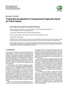
Figure 1 – Pairwise neighbour densities and local correlation patterns, simulated data .

data, the results were unaltered. As null distribution we used a normal bivariate distribution with correlation equal to zero. In Figure 1 pairwise neighbour densities and local correlations are plotted against the radius (∆r = 0.05). As expected distances between data points belonging to two highly related predictor variables (x and g) were different from those between the other pairs. This seems to indicate that in the case of multicollinearity which leads to approximate concurvity, this nonparametric approach based on maximal local correlation succeeds to detect global nonlinear relationships between predictors.

On concurvity in nonlinear and nonparametric regression models

93

TABLE 3 Boston Housing dataset

Label CRIM ZN INDUS CHAS NOX RM AGE DIST RAD TAX PTRATIO B LSTAT

Description per capita crime rate by town proportion of residential land zoned for lots over 25,000 sq.ft. proportion of non-retail business acres per town Charles River adjacency nitric oxides concentration (parts per 10 million) average number of rooms per dwelling proportion of owner-occupied units built prior to 1940 weighted distances to five Boston employment centres index of accessibility to radial highways full-value property-tax rate per $10,000 pupil-teacher ratio by town (Bk − 0.63)2 , where Bk is the proportion of blacks by town % lower status

MEDV

median value of owner-occupied homes in $1000’s

6.

Real data: Boston Housing

The data set used in this section is called the Boston Housing dataset. It was originally collected by Harrison and Rubingeld (1978) and was used to estimate the air pollution effect on housing values in suburbs of Boston. This dataset contains 506 instances on 14 variables (13 continuous variables and a binary one) and there are no missing values. The variables are reported in Table 3. The dependent variable is MEDV and it indicates the median value of owner-occupied homes in $1000’s. Drawing from an example proposed in (Donnell et al., 1994) we will examine the behaviour of the maximal local correlation statistics on the full dataset and on a reduced one proposed by Breiman and Friedman (1985). The reduced dataset contains 5 predictors: 4 chosen via forward stepwise variable selection (RM, TAX, PTRATIO and LSTAT) and NOX to evaluate the effect of air pollution. In Table 4 the eigenvalues of the correlation matrix of the independent variables and the values of tolerance are shown. We can notice that the full dataset is badly conditioned, especially if we look at the values of tolerance for the predictors RAD and TAX.

6.1.

Reduced dataset: Boston Housing data

In Table 5 maximal local correlation statistics are reported. As in the previous analysis the two-sided p-values were evaluated via permutation test with 1000 replications. The rate of change of the radius used was equal to ∆r = 0.05. As null distribution we used a simulated normal bivariate distribution whose correlation was equal to zero. We can notice that maximal local correlation statistics are

S. Amodio, M. Aria and A. D’Ambrosio

94

TABLE 4 Eigenvalues of the correlation matrix and tolerance of the predictors, Boston Housing data

CRIM ZN INDUS NOX RM AGE DIS RAD TAX PTRATIO B LSTAT

Eigenvalues 6.1267 1.3425 1.1798 0.8351 0.6647 0.5374 0.3964 0.2771 0.2203 0.1862 0.1693 0.0646

Tolerance 0.5594 0.4351 0.2532 0.2279 0.5176 0.3233 0.2528 0.1352 0.1127 0.5608 0.7435 0.3412

TABLE 5 Maximal local correlation, Boston Housing reduced data NOX RM TAX PTRATIO

NOX 1.0000

RM 0.2648

TAX 0.6077

PTRATIO 0.5616

LSTAT 0.3789

(0.3567)

(0.0320)

(0.0367)

(0.1521)

1.0000

0.3585

0.2562

0.3812

(0.1567)

(0.5876)

(0.1498)

1.0000

0.5655

0.2179

(0.0331)

(0.5438)

1.0000

0.2008 (0.6136)

LSTAT

1.0000

On concurvity in nonlinear and nonparametric regression models

95

TABLE 6 Maximal local correlations, Boston Housing Complete data CRIM ZN INDUS NOX RM AGE DIS RAD TAX PTRATIO B LSTAT

CRIM 1.000

ZN 0.275 1.000

INDUS 0.586 0.419 1.000

NOX 0.664 0.285 0.784 1.000

RM 0.308 0.241 0.342 0.164 1.000

AGE 0.554 0.313 0.424 0.657 0.298 1.000

DIS 0.549 0.348 0.533 0.665 0.313 0.706 1.000

RAD 0.488 0.247 0.480 0.439 0.166 0.190 0.222 1.000

TAX 0.476 0.206 0.610 0.504 0.309 0.347 0.466 0.387 1.000

PTRATIO 0.382 0.214 0.502 0.446 0.186 0.306 0.335 0.438 0.395 1.000

B 0.219 0.134 0.212 0.258 0.226 0.185 0.198 0.269 0.218 0.161 1.000

statistically significant at significance level α = 0.05 for NOX - TAX, NOX PTRATIO and TAX - PTRATIO. Note that this result is extremely close to the one obtained in Donnell (1982) using APCs.

6.2.

Complete data set: Boston Housing data

Maximal local correlation statistics for the complete dataset are shown in Table 6.

ZN

INDUS

NOX

RM

AGE

DIS

RAD

TAX

PTRATIO

B

LSTAT

TAX

PTRATIO

B

LSTAT

CRIM

DIS

0.657

0.706

0.664

0.784

CRIM

ZN

INDUS

NOX

RM

0.665

AGE

RAD

0.61

0.0

0.2

0.4

0.6

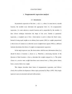
Figure 2 – Maximal local correlation statistics, Boston Housing complete data

In Figure 2 the highest statistically significant maximal local correlation statistics are highlighted. We can notice that the proposed methodology succeeds in finding nonlinear associations between the following predictors: TAX - INDUS, DIS - NOX, DIS - AGE, AGE - NOX, NOX - CRIM, NOX - INDUS. Also these results are similar to the ones obtained in Donnell (1982) using APCs. This indicates again that in the case of badly conditioned input matrix, this nonparametric approach based on maximal local correlation succeeds in spotting global nonlinear relationships between untransformed predictors.

LSTAT 0.218 0.224 0.280 0.326 0.338 0.322 0.194 0.149 0.177 0.151 0.119 1.000

S. Amodio, M. Aria and A. D’Ambrosio

96

7.

Concluding remarks

In this study, we have demonstrated that the proposed nonparametric approach based on maximal local correlation statistics succeeds in detecting global nonlinear relationships between predictor variables. For this reason we believe that it can be used as a perspective or as a retrospective diagnostic for concurvity especially in real data cases. Indeed, in these cases, concurvity tends to be present when predictor variables show strong association patterns. Moreover this approach can be used, together with the other diagnostics, as a variable selection method before implementing an additive model. A natural extension of this study would be to test the efficacy and the efficiency of this method when nonlinear association among predictors is characterized by the presence of clusters within the data. ACKNOWLEDGEMENTS We would like to thank the anonymous referee for his or her extremely useful suggestions. REFERENCES R. E. Bellman (1961). Adaptive control processes: a guided tour, vol. 4. Princeton university press Princeton. L. Breiman, J. H. Friedman (1985). Estimating optimal transformations for multiple regression and correlation. Journal of the American Statistical Association, 80, no. 391, pp. 580–598. A. Buja, T. Hastie, R. Tibshirani (1989). Linear smoothers and additive models. The Annals of Statistics, pp. 453–510. ¨ ller, R. J. Carroll, Y. A. Chen, J. S. Almeida, A. J. Richards, P. Mu B. Rohrer (2010). A nonparametric approach to detect nonlinear correlation in gene expression. Journal of Computational and Graphical Statistics, 19, no. 3, pp. 552–568. J. De Leeuw, F. W. Young, Y. Takane (1976). Additive structure in qualitative data: An alternating least squares method with optimal scaling features. Psychometrika, 41, no. 4, pp. 471–503. D. J. Donnell (1982). Additive principal components - a method for estimating equations with small variance from data. Ph.D. thesis, University of Washington, Seattle. D. J. Donnell, A. Buja, W. Stuetzle (1994). Analysis of additive dependencies and concurvities using smallest additive principal components. The Annals of Statistics, pp. 1635–1668. P. H. Eilers, B. D. Marx (1996). Flexible smoothing with b-splines and penalties. Statistical science, pp. 89–102.

On concurvity in nonlinear and nonparametric regression models

97

J. H. Friedman (1997). On bias, variance, 0/1-loss, and the curse-ofdimensionality. Data mining and knowledge discovery, 1, no. 1, pp. 55–77. J. H. Friedman, W. Stuetzle (1981). Projection pursuit regression. Journal of the American statistical Association, 76, no. 376, pp. 817–823. P. Grassberger, I. Procaccia (1983). Characterization of strange attractors. Physical review letters, 50, no. 5, pp. 346–349. P. J. Green, B. W. Silverman (1993). Nonparametric regression and generalized linear models: a roughness penalty approach. CRC Press. C. Gu (1992). Diagnostics for nonparametric regression models with additive terms. Journal of the American Statistical Association, 87, no. 420, pp. 1051– 1058. C. Gu, D. M. Bates, Z. Chen, G. Wahba (1989). The computation of generalized cross-validation functions through householder tridiagonalization with applications to the fitting of interaction spline models. SIAM Journal on Matrix Analysis and Applications, 10, no. 4, pp. 457–480. C. Gu, G. Wahba (1991). Minimizing gcv/gml scores with multiple smoothing parameters via the newton method. SIAM Journal on Scientific and Statistical Computing, 12, no. 2, pp. 383–398. H. Gu, T. Kenney, M. Zhu (2010). Partial generalized additive models: An information-theoretic approach for dealing with concurvity and selecting variables. Journal of Computational and Graphical Statistics, 19, no. 3, pp. 531– 551. T. Hastie, R. Tibshirani (1986). Generalized additive models. Statistical science, 1, no. 3, pp. 297–310. T. J. Hastie, R. J. Tibshirani (1990). Generalized additive models, vol. 43. CRC Press. G. W. Stewart (1987). Collinearity and least squares regression. Statistical Science, 2, no. 1, pp. 68–84. C. J. Stone (1985). Additive regression and other nonparametric models. The annals of Statistics, pp. 689–705. G. Wahba (1990). Spline models for observational data, vol. 59. Siam.

SUMMARY On concurvity in nonlinear and nonparametric regression models When data are affected by multicollinearity in the linear regression framework, then concurvity will be present in fitting a generalized additive model (GAM). The term concurvity describes nonlinear dependencies among the predictor variables. As collinearity

98

S. Amodio, M. Aria and A. D’Ambrosio

results in inflated variance of the estimated regression coefficients in the linear regression model, the result of the presence of concurvity leads to instability of the estimated coefficients in GAMs. Even if the backfitting algorithm will always converge to a solution, in case of concurvity the final solution of the backfitting procedure in fitting a GAM is influenced by the starting functions. While exact concurvity is highly unlikely, approximate concurvity, the analogue of multicollinearity, is of practical concern as it can lead to upwardly biased estimates of the parameters and to underestimation of their standard errors, increasing the risk of committing type I error. We compare the existing approaches to detect concurvity, pointing out their advantages and drawbacks, using simulated and real data sets. As a result, this paper will provide a general criterion to detect concurvity in nonlinear and non parametric regression models. Keywords: Concurvity; multicollinearity; nonparametric regression; additive models; generalized additive models.