On Digit-by-Digit Methods for Computing Certain Functions

On

Digit-by-Digit Methods for Computing Certain Functions Milo-s D. Ercegovac Computer Science Department Univ. of California at Los Angeles

Abstract- A digit-by-digit arithmetic method in computing certain functions, such as cube roots, suitable for FPGA technologies, is presented. In the radix-2 case, this method uses only simple primitive operations such as carry-propagate addition/subtraction, doubling, and halving. Details of the radix-2 method applied to computing cube root and its square are discussed. Rough estimates of delay and cost are given.

INTRODUCTION The scope of current and forthcoming technologies is enlarging. Besides semi- and full-custom VLSI, reconfigurable ICs, based on the concept of field-programmable gate arrays (FPGA), are becoming suitable for digital system design and implementation when the expected volume and life time are limited. However, FPGA technology has constraints and characteristics different from other VLSI integrated circuits. For these reasons it may be profitable to revisit approaches to design of arithmetic schemes. In this paper we consider a class of algorithms which might be suitable for FPGA implementations. We discuss a digit-by-digit method, in which operands and/or results are processed digit-at-a-time. These have been used often when simplicity is needed in interconnections and in arithmetic circuits while increases in latency, due to serial processing, are acceptable [4]. These characteristics were common in the early days of computer design and it may be instructive to look at some of the early approaches to implementing arithmetic operations. Specifically, we revisit rather old ideas for computing inverses of certain functions [8], [12] and adapt them for implementation using field-programmable gate arrays. As mentioned above, this technology has different constraints and features than custom VLSI. A most relevant difference is in implementing adders. While fast adders in custom VLSI use sophisticated schemes such as parallel prefix adders, in an FPGA a basic carry-ripple adder is often preferable because of the built-in carry paths between neighboring configurable blocks and compact mapping. These dedicated carry paths have much shorter delay than the general routing channels which would be used in implementing more elaborate adders. Consequently, many of the adder schemes developed for custom VLSI do not map well to FPGAs. In particular, redundant adders may not be attractive in terms of delays and area compared to simple carry-propagate adders such as the carry-ripple adder which has built-in support on FPGAs. On the other hand, FPGA lookup table (LUT) logic blocks allow efficient implementation of multi-operand reduction which can be combined with fast carry-ripple adder to implement, for

978-1-4244-2110-7/08/$25.00 C2007 IEEE

338

example [3:1] adders. In general, as long as reductions, such as [3;2] (carry-save), are confined to internal logic and avoid global interconnect, their use is advantageous. An example of such a design is supported by the Altera's adaptive logic module (ALM) which consists of 4 3-input LUTs performing a carry-save reduction of 3 to 2 operands and a 2-bit CRA with a fast carry propagation chain [1]. Thus, the ALMs implement efficiently a [3:1] adder. Suggestions for improving carry-propagation schemes in FPGAs have been studied in [5]. Early approaches for implementing arithmetic operations and evaluation of functions often utilized digit-by-digit methods. Examples of well-known methods of this type are digitrecurrence division and square root [2], CORDIC [11], multiplicative and additive normalization methods for logarithms and exponentials, and online arithmetic [3]. These early arithmetic approaches used conventional (nonredundant) arithmetic and were not attractive in custom VLSI. However, these approaches may be of interest because modern technologies such as FPGAs may favor conventional representations. I. OVERVIEW OF THE METHOD

Folowing Morrison [8] and Wensley [12], consider computing the inverse of a function f (x) = y satisfying the following properties: 1) f(x) = y is non-decreasing in the interval where we want to obtain the inverse x = f-(y) 2) f (x) is additive, i.e., f (a + b) = G(f (a), b) For the conventional radix-2 system the partially computed result at iteration i, containing i digits, is represented as

x[i]

=

xj2 -j,

xi C {O, 1}

(1)

j=l

If x[i] < x < x[i] + 2-i then the following holds because f (x) is a non-decreasing function: 1) x[i] < x < x[i] + 2-(i±+) if f(x[i] + 2-(i±+)) > y 2) x[i] + 2-(i±+) < x < (x[i] + 2-(i±+)) + 2-(i±+) if f (x[i] + 2-(i±+)) < y Calculation of fnext = f(x[i] + 2-(i±+)), given f(x[i]), uses function G, which, hopefully, is simpler than using f (x) directly to compute fnext. The next result digit is determined so that the error Cnext = Y-fnext satisfies a desired condition. A simple condition is to keep the error nonnegative. This is a well-known condition used in restoring (nonperforming)

division.

A general algorithm for radix-2 system with xj C {0, 1} is for j = 0,..., m Ido 1. fnext f(x[j] + 2-(j+l)) = G(f(x[j], 2-(j+l)) y 2. e[j + fnext 3. x[j +1= (x[j, (e[j + 1] > 0) x 2 -(j+)) so that x[m] ) f -(y) as m )co. The main objective in developing an algorithm suitable for hardware implementation is to find simple ways to carry out Step 1. One simple solution is to decompose G into several functions which are simpler to implement than f(x). In the next section we illustrate the algorithm development using an example - computing a cube root and its square.

The corresponding recurrences are obtained from definitions by considering the possible values of the next result digit xj+x. For a [j] = (y- (x [j])3 ) /dj+ I we get the following recurrence:

II. COMPUTING CUBE ROOT AND CUBE ROOT SQUARE Digit-recurrence algorithms for computing cube roots have been considered frequently in the literature. Examples of work

b[j] + xj+l(2c[j] + xj+lPj)

include [9], [7], [6]. Typical for the approaches proposed is the use of redundant result digit sets and residuals in redundant form to simplify the result digit selection and reduce the time per iteration. These improvements come at the cost of extra hardware compared with methods not using redundancy. As indicated earlier, in this paper we focus on the algorithms based on conventional (nonredundant) systems - specificaly radix-2 [12]. Let f(x) = x3 = y, 0 < y < 1, and compute x = y1/3. The result is m

x Z=

xjCf0,1}

xi2-, i=O

At step j, we want to compute x[j + 1] = x[j] + xj+12 (j+1) = (x[j],xj+±). Let di = 2- and the error

(residual)

e[j]

=

y -[j]

(2)

The next result digit xj+l is selected so that e[j + 1] > 0, i.e., xj+= (e[jl 1] > 0). A suitable expression for the error can be obtained as follows. Compute the error for xj+l = 1 y -(x[j] + dj+±)

-(x[j]) -3(x[j])2dj+± -3x[j]dX2+i- d3+

y

Divide (3) by dj+l and define the terms that define corresponding scaled residual expression as a [j]

=

b[j]

c[j]

(y- (x[j])3)Idj+l (X[j])2 x[j]dj+

d2j+ 1 pj Now the scaled residual w[j + 1] is expressed as

a[j] -3b[j] -3c[j] -pj (4) Instead of computing the next residual using the current residual, the terms a[j + 1], b[j + 1], c[j + 1], and Pj+l are computed separately and combined to form the next residual. w[j + 1]

=

339

a [j +

1]

= =

=

(y- (x[j + 1])3)/dj+2

(Y-(x[j] + xj+ldj+±)3)Idj+2

2(a[j]- xj+l (3b[j] + 3c[j] + pj))

(x[j])2 the recurrence is: (X[j +1])2 b[j + 1]

For b[j]

=

(X[j] + Xj+ldj+1)2

(X[j])2 + 2x[j]xj+ldj+l For c[j]

x[j]dj +

+

(Xj+1)2(dj +)2

the recurrence is:

(x[j + 1])dj+2

c[j + 1]

(x[j] + xj+ldj+±)dj+112 I2 (X[j]dj+i H-j+, (dj+1)2) =

2(c[j] + xj+lPj)

These recurrences use additions, subtractions, left and right shifts by one or two positions, and powers of 2. The range of the terms are: 0 < a[j] < 6, 0 < b[j] < 1, and 0 < c[j] < 2-(j+1). The range of the scaled residual is -3 < w[j] < 3. In the radix-2 case, we compute tentative scaled residual for Xj+1 = 1

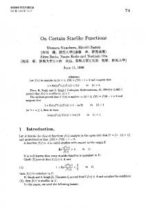
w[j + 1] = a[j] -3b[j] -3c[j] -pj and then use its sign to select the result digit xj+ f 1 if w[j+l1]>0 XJj4 ' 0 otherwise This is equivalent to computing a tentative remainder in digit-recurrence division and, based on the sign, updating the next remainder and the quotient. The difference in this case is that the next residual is not computed directly from the tentative residual. The algorithm for radix-2 cube root and its square is summarized next. 1. Intialization: a[O] = 2y; b[O] = 0; c[O] = 0; do 1; Po =; x[0]= 0 2. Forj =0,...,m -Ido 2.1 w[j + 1] = a[j] -3(b[j] + c[j]) -pj 2.2 if w[j + 1] > 0 then a[j + 1] = 2w[j + 1] b[j + 1] = b[j] + 2c[j] +pj c[j+1] = 2 (c[j] + pj) X[j+ 1] = (x[j],1) 2.3 else a[j + 1] = 2a [ji b[j + 1] = b[j] c[j + 1] = 1c[j] x[j + 1] = (x[j], 0) 2.4 pj+I = 1pj; dj+2 = 2dj+

i w[j + 1] 00.0 01.01

0

1

2 3 4 5 6 7 8

9 10 11

12

Xj+l

0

01.0101 00.101001 -01.00101111 00.0010111011 -10.001001000011 -01.110000010011 -01.000000111 00.01110011111 -01.10010010011 -00.1010101001 01.001001011

1

1

1

0

1 0 0 0

1 0 0 1

a[j + 1]

x[j + 1] 0.0 0.1

b[j + 1]

01.1 10.1

0.11 0.111 0.111 0.11101 0.11101 0.11101 0.11101

0.111010001

0.111010001 0.111010001

0.111010001001

10.101 01.01001 10.1001 00.010111011 00.10111011 01.0111011 10.111011 00.11100111110 01.110011111001 11.10011111001 10.01001011

0.0 0.01

0.1001

0.110001 0.1101001001

0.1101001001 0.1101001001 0.1101001001

0.1101001001

0.110100110011

0.110100110011 0.11010011001 0.1101001101

Fig. 1. Example of cube root computation. The argument y = 0.75 and the result x = y1/3 = 0.9085 = 0.111010001001 truncated to 12 fractional places. The computed result is x[12] = 0.111010001001 with an error of less than one ulp. We also obtain z = x2 =y2/3 = 0.110100110101 computed as b[12] = 0.110100110100.

3. Outputs: x x[m]; 92 - b[m] An example is shown in Figure 1. Note that b[rn] -_ y2/3. The algorithm uses simple operations: left/right shifts, addition and subtraction. The overall scheme consists four modules: Module 1, shown in Figure 2, produces w's, the result digit xj+i, and a's. -

b

An alternative implementation of Module 1 using a [3:1] adder is illustrated in Figure 3.

Module ] Stepj

b

c

Stepj

-a

-w =-a + 3(b+c) + p

anext = 2a or 2w

Fig. 3. Alternative implementation for Module 1.

-a

-w =-a+ 3(b+c) + p

anext = 2a or 2w

Fig. 2. Implementation scheme for cube root: Module 1.

To simplify the implementation we compute a negative of the residual w[j+1], i.e., -w[j+] =-a[j]+pj+3(b[j]+c[j]) and keep a[j] in the negative form, thus avoiding subtraction. The term -a[j + 1] =-2a[j] or -a[j + 1] -2w[j + 1], depending on the sign. The output digit xj+l 1 if the sign s < U and O otherwise. So, the register Reg-A is loaded with -2w[j + 1] if xj+l = 1 and shifted otherwise. The Append operation adds a 1( pj = 2 -2(j+l)) in even positions. The output of this operator is shared among modules using Pj+1.

340

Modules 2 and 3, shown in Figure 4, produce terms b[j + 11 and c[j + 1] and store them in the corresponding registers in a similar manner as discussed for Module 1. Module 4 is a shift register which updates the result x[j + 1] = (x[j], xj+l) using concatenation. The results are obtained in a conventional representation. The CPA adders and INC incrementers in Figure ?? propagate carries in an overlapped manner so that the total latency is roughly the latency of a single CPA (INC) module. The cycle time is estimated as

Tcycle

-

(m + 3)tcarry + 3tFA + tREG

The cost is estimated using the area of a full adder AF

Module 2 b

2c

outputs. The following are the expressions for the conditional terms:

Module 3

a°° [j + 2] boo [j + 2] COO [j + 2] Xj+]

ao0[j -+ 2]

bo0

b

bnext = b+2c +p or b Fig. 4.

[j + 2] -+ 2]

c01[j

a1o[j -+ 2] b1o[j -+ 2] c10[j + 2]

-

OVERLAPPED STAGES: 2 BITS/PER CYCLE

Two result bits xj+l and Xj+2 can be obtained per cycle by using two overlapped stages [10], [2], a scheme used in speeding up digit-recurrence division. An overall scheme of this alternative in implementing cube root scheme is shown in Figure 5. The inputs to the combined stages are a[j], b[j], c[j], and the iteration index j. The block BI computes w[j -+ 1] = a[j]- 3(b[j] + c[j]) -pj and outputs the result digit xj+x. In parallel blocks B2 and B3 produce two conditional next residuals wo[j + 1] and w1[j + 2] for xj+ = 0 and xj+ = 1, respectively. The tentative residuals are used to determine tentative values of the next result digit x°2 and x+2. The tentative residuals are

2a[j]- 3(b[j] + c[j]2 1) -Pj+ 2w[j + 1] -3(b[j] + 2c[j] +pj) -Pj+l

w° [j + 2] w1[j + 2]

Block B4 computes the tentative values of

and c[j + 2]

(a°°[j

a

[j

2],

b [j

2],

as:

-+

c[j]2 -2

2w° [j + 2] b[j] + c[j] + pj+i c[j]2-2 +pj2 -3

=

4w[j + 1] b[j]

=

c[j]2 -2

=

(7m + 1O)AFA

Further optimizations include shared CPA/INC modules to reduce the cost at an increased cycle time. To reduce latency other types of conventional adders, such as carry-skip and carry-select adders, could be considered, as discussed in [13], [5]. Another possibility is a scheme with overlapped stages outlined in the next section. III.

=

(c +p)/2 or c/2

cnext

Implementation scheme for cube root: Modules 2 and 3.

C

=

4a[j] b[j]

=

2], ao1[j -+ 2], a10[j + 2], a" [j + 2])

(boo[j + 2], bo1[j + 2], bl0[j + 2], bl1[j + 2]) (cOO[j + 2],c01[j + 2],c10[j + 2],c" [j + 2])

The values of the result digit pair which of these conditional terms

(Xj+l, Xj+2)

are

selected

as

determine the stage

341

all [j + 2] b1l [j + 2] c1l [j + 2]

2w° [j + 2] b[j] + 2c[j] + Pj (c[j] +pj)2 -2

The conditional forms of the terms a, b, and c are computed with shifts which are done via wiring and additions which depend on the stage inputs so Block 4 is not in the critical path. The delay of Blocks 1, 2 and 3 is roughly equivalent to the delay of radix-2 stage (less the register delay. Therefore, the overlapped stage delay is roughly the delay of a single stage plus the delay of a 4-to-I selector and the delay of registers for a, b, and c terms. We ignore the implementation of p terms. In conclusion, two bits are computed per iteration with a delay of a single stage discussed above. However, there is an increase in the cost of this implementation: we estimate that it would take about five times as much hardware as the one bit per stage implementation. IV. SUMMARY We have reviewed and expanded on a simple approach to digit-by-digit methods, originally proposed by Morrison and Wensley in the 50s. This approach is of interest when conventional adders are "best" as is often the case in current FPGA technologies. The method is applicable to other functions such square root, division, logarithm, exponential, arctangent, arcsin, and similar. The method has been illustrated in computing the cube root and its square in radix2 conventional representation without use of redundancy. A 2-bit per iteration alternative has been discussed. Estimates of delays and cost are given. No synthesis has been done so the performance results are rough estimates. It may be useful to consider extensions to higher radices with redundant digit sets to allow simple comparison constants while still employing carry-propagate adders as used in the SRT division with nonredundant residuals [3].

aft] bfj] cfj]

XjO+2 IFXj+2

oE

|

+ Block B4 (x4) |(x4) |(x4) | t t

Xj+ I

Xj+2

a[j+2]

l conditional

~~tetrms a, b, and c

bfj+2] cj+2]

Fig. 5. Scheme with two overlapped stages.

REFERENCES [1] Altera Corporation. Stratix III Device Handbook, Volume 1. October 2007. [2] M. D. Ercegovac and T. Lang. Division and Square Root: DigitRecurrence Algorithms and Implementations. Kluwer Academic Publishers, Boston, MA, 1994. [3] M.D. Ercegovac, T. Lang, Digital Arithmetic, San Francisco, Morgan Kaufmann, 2004. [4] R. Hartley and K. Parhi. Digit-Serial Computation. Springer, 1995. [5] S. Hauck, M.M. Hosler, and T. W. Fry. High-Performance Carry Chains for FPGAOs. IEEE Trans. On Very Large Scale Integration (VLSI) Systems, 8( 2):138-147, April 2000. [6] P. Montuschi, J. D. Bruguera, L. Ciminiera, J-A. Pineiro. A Digitby-Digit Algorithm for mth Root Extraction. IEEE Trans. Computers, 56(12):1696-1706, December 2007. [7] J.A. Pineiro, J.D. Bruguera, L. Ciminiera, P. Montuschi. A Digit-by-Digit Algorithm for Radix-2 Cube Root and Its Implementation. Technical Report, May 2004, http://www.ac.usc.es/arquivos/articulos/2004/gac2004-iOl.pdf. [8] D.R. Morrison. A Method for Computing Certain Inverse Functions. MTAC, Vol. 10, No. 56, pp. 202-208. [9] N. Takagi. A Digit-Recurrence Algorithm for Cube Rooting. EICE Transactions on Fundamentals of Electronics, Communications and Computer Sciences. Vol.E84-A, No.5, pp.1309-1314, 2001. [10] G.S. Taylor. Radix-16 SRT Dividers with Ovelapped Quotient-Digit Stages. Proc. 7th IEEE Symposium on Computer Arithmetic, pp. 6471, 1985. [11] J. S. Walther. A unified algorithm for elementary functions. In Joint Computer Conference Proceedings, pages 379-387, 1971. Reprinted in E. E. Swartzlander, Computer Arithmetic, Vol. 1, IEEE Computer Society Press, Los Alamitos, CA,1990. [12] J. H. Wensley. A Class of Non-Analytical Iterative Processes. The Computer Journal, Vol. 2, pp. 163-167, 1959. [13] S. Xing and W.W.H. Yu. FPGA Adders: Performance Evaluation and Optimal Design. IEEE Design & Test Of Computers, pp.24-29, JanMarch 1998.

342