ON DIMENSIONALITY REDUCTION FOR ... - CiteSeerX

ON DIMENSIONALITY REDUCTION FOR CLASSIFICATION AND ITS APPLICATION Raviv Raich† , Jose A. Costa‡ , and Alfred O. Hero III† †

‡

Department of EECS, University of Michigan, Ann Arbor, MI 48109-2122, USA Center for the Mathematics of Information, California Institute of Technology, Pasadena, CA 91125, USA

ABSTRACT In this paper, we evaluate the contribution of the classification constrained dimensionality reduction (CCDR) algorithm to the performance of several classifiers. We present an extension to previously introduced CCDR algorithm to multiple hypotheses. We investigate classification performance using the CCDR algorithm on hyperspectral satellite imagery data. We demonstrate the performance gain for both local and global classifiers and demonstrate a 10% improvement of the k-nearest neighbors algorithm performance. We present a connection between intrinsic dimension estimation and the optimal embedding dimension obtained using the CCDR algorithm. 1. INTRODUCTION In classification, the goal is to find a mapping from the domain X to one of several hypotheses based on observations that lie in X . In some problems, the observations from the domain X lie on a manifold in X with a dimension lower or equal to that of X (e.g., the unit circle in the x-y plane or the x-axis in the x-y plane). Whitney’s theorem states that every smooth d-dimensional manifold admits an embedding into 2d+1 . This motivates the approach taken by kernel methods such as support vector machines [1]. Clearly, there exist an embedding to a higher dimensional space (i.e., 2d+1 ). Our interest is in finding an embedding into a lower dimensional space.

R

R

8 6 4

e1

2 0

e2

−2 −4 −6 −8 −8

−6

−4

−2

0

2

4

6

8

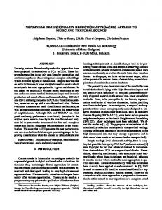
Fig. 1. PCA of a two-classes classification problem. Dimensionality reduction of high dimensional data, was addressed in classical methods such as principal component analysis (PCA) [2] This work was partially funded by the DARPA Defense Sciences Office under Office of Naval Research contract #N00014-04-C-0437. Distribution Statement A. Approved for public release; distribution is unlimited.

and multidimensional scaling (MDS) [3, 4]. In PCA, an eigendecomposition of the d × d empirical covariance matrix is performed and the data points are linearly projected along the m ≤ d eigenvectors with the largest eigenvalues. A problem that may occur with PCA for classification is demonstrated in Fig. 1. When the information that is relevant for classification is present only in the eigenvectors associated with the small eigenvalues (e2 in the figure), removal of such eigenvectors may result in severe degradation in classification performance. In MDS, the goal is to find a lower dimensional embedding of the original data points that preserves the relative distances between all the data points. The two methods suffer greatly when the manifold is nonlinear. For example, PCA will not be able to offer dimensionality reduction for classification of two classes lying each on one of two concentric circles. In the seminal paper of Tenenbaum et al [5], Isomap, a global dimensionality reduction algorithm was introduced taking into account the fact that data points may lie on a lower dimension manifold. Unlike for MDS, geodesic distances (distances that are measured along the manifold) are preserved by Isomap. Belkin and Niyogi present a related Laplacian eigenmaps dimensionality reduction algorithm in [6]. The algorithm performs a minimization on the weighted sum of squared-distances of the lower-dimensional data. Each weight multiplying the squared-distances of two low-dimensional data points is inversely related to distance between the corresponding two highdimensional data points. The algorithms mentioned above consider the problem of learning a lower-dimensional embedding of the data. In classification, such algorithms can be used to preprocess high-dimensional data before performing the classification. This could potentially allow for a lower computational complexity of the classifier. In some cases, dimensionality reduction results in increased computational complexity of the classifier. To guarantee a low computational complexity of the classifier of the low-dimensional data, a classification constrained dimensionality reduction (CCDR) algorithm was introduced in [7]. The CCDR algorithm is an extension of Laplacian eigenmaps [6] and it incorporates class label information into the cost function, reducing the distance between points with similar label. In [7] the CCDR algorithm was only studied for two classes and its performance was illustrated for simulated data. In this paper, we introduce an extension of the algorithm to the multi-class problem and present experimental results for the Landsat MSS imagery data [8]. We study the algorithm performance as its various parameters, (e.g., dimension, label importance, and local neighborhood), are varied. We study the performance of CCDR as preprocessing prior to implementation of several classification algorithms such as k-nearest neighbors, linear classification, and neural networks. We demonstrate a 10% improvement over the k-nearest neighbors algorithm performance benchmark for this dataset. We address the issue of dimension estimation and its effect on classification performance. The organization of this paper is as follows. Section 2 presents

the multiple-class CCDR algorithm. Section 3 provides a study of the algorithm using the Landsat dataset and Section 4 summaries our results. 2. CLASSIFICATION CONSTRAINED DIMENSIONALITY REDUCTION

3. ALGORITHM STUDY In this section, we present a performance study of three classical classification algorithms on data after CCDR preprocessing. First, we provide a brief description of the algorithms.

Here, we review the CCDR algorithm [7] and extend it to multi-class classification. Let Xn = {x1 , x2 , . . . , xn } be a set of n points constrained to lie on an m-dimensional submanifold M ⊆ d . Each point xi ∈ M is either associated with a class label, i.e., xi has label ci ∈ {A1 , A2 , . . . , AL }, or is unlabeled. Our goal is to obtain a lowerdimensional embedding Yn = {y 1 , y 2 , . . . , y n } (where y i ∈ m with m < d) that preserves local geometry while clustering points with the same labels to improve the performance of classifiers based on the lower-dimensional data. First, an adjacency matrix W is constructed as follows: For k ∈ , a k-nearest neighbors graph is constructed with the points in Xn as the graph vertices. Each point xi is connected to its knearest neighboring points. For a fixed scale parameter ǫ > 0, the weight ˘ associated with¯ the two points xi and xj satisfies wij = exp −kxi − xj k2 /ǫ if xi and xj are connected and wij = 0 otherwise. To cluster points of the same label we associate each class with a class center namely z k ∈ m . Let C be the L×n class membership matrix with the ki-th element cki = 1 if ci = Ak and cki = 0 otherwise. If xi is unlabeled then cki = 0 for all k. We construct the following cost function: X βX J(ZL , Yn ) = wij ky i − y j k2 , (1) cki kz k − y i k2 + 2 ij

R

R

N

(a) PCA

R

ki

where ZL = {z 1 , . . . , z L } and β ≥ 0 is a regularization parameter. Large values of β produce an embedding that ignores class labels and small values of β produce an embedding that ignores the manifold structure. Our goal is to find ZL and Yn that minimize the cost function in (1). Let Z = [z 1 , . . . , z L , y 1 , . . . , y n ], I be the L × L identity matrix and » – I C W′ = . C T βW Minimization over Z of the cost function in (1) can be expressed as “ ” min tr ZLZ T , (2) ZD1 = 0 ZDZT = I

where D = diag(W ′ 1) and L = D − W ′ . To prevent the lowerdimensional points and the class centers from collapsing into a single point at the origin, the regularization ZDZ T = I is introduced. The second constraint ZD1 = 0 is constructed to prevent a degenerate solution, e.g., z 1 = . . . = z L = y 1 = . . . = y n . This solution may occur since 1 is in the null-space of the Laplacian L operator, i.e., L1 = 0. The solution to (2) is Z that satisfies the generalized eigendecomposition given by LZ

T

T

= DZ diag(λ).

(3)

Specifically, matrix Z is given by the generalized eigenvectors associated with the m smallest positive generalized eigenvalues, where the first rows correspond to the coordinates of the class centers and the following rows determine the embedding of the original data points.

(b) CCDR

Fig. 2. Three-dimensional projection of the (a) PCA and (b) CCDR lower-dimensional embedding of the Landsat MSS satellite imagery dataset. Classes 1, 2, 3, 4, 5, and 6, are marked with ×, ◦, +, ⋄, △, and ⋆, respectively. Test data points are marked by dots.

3.1. Classification Algorithms We consider three widespread algorithms: k-nearest neighbors, linear classification, and neural networks. A standard implementation of k-nearest neighbors was used, see [1, p. 415]. The linear classifier we implemented is given by

ˆ

cˆ(y)

=

arg

(Ak ) ˜

=

arg min

α(Ak ) , α0

max

c∈{A1 ,...AL }

[α,α0 ]

(c)

y T α(c) + α0

n X (y Ti α + α0 − cki )2 , i=1

for k = 1, . . . , L. The neural network we implemented is a threelayer neural network with d elements in the input layer, 2d elements in the hidden layer, and 6 elements in the output layer (one for each class). Here d was selected using the common PCA procedure, as the smallest dimension that explains 99.9% of the energy of the data. A gradient method was used to train the network coefficients with

3.2. Data Description In this section, we examine the performance of the classification algorithms on the benchmark label classification problem provided by the Landsat MSS satellite imagery database [8]. Each sample point consists of the intensity values of one pixel and its 8 neighboring pixels in 4 different spectral bands. The training data consists of 4435 36-dimensional points of which, 1072 are labeled as 1) red soil, 479 as 2) cotton crop, 961 as 3) grey soil, 415 as 4) damp grey soil, 470 are labeled as 5) soil with vegetation stubble, and 1038 are labeled as 6) very damp grey soil. The test data consists of 2000 36-dimensional points of which, 461 are labeled as 1) red soil, 224 as 2) cotton crop, 397 as 3) grey soil, 211 as 4) damp grey soil, 237 are labeled as 5) soil with vegetation stubble, and 470 are labeled as 6) very damp grey soil. In the following, each classifier is trained on the training data and its classification is evaluated based on the entire sample test data. In Table 1, we present “best case” performance of neural networks, linear classifier, and k-nearest neighbors in three cases: no dimensionality reduction, dimensionality reduction via PCA, and dimensionality reduction via CCDR. The table presents the minimum probability of error achieved by varying the tuning parameters of the classifiers. The benefit of using CCDR is obvious and we are prompted to further evaluate the performance gains attained using CCDR. No dim. reduc. PCA CCDR

Neural Net. 83 % 9.75 % 8.95 %

Lin. 22.7 % 23 % 8.95 %

k-nearest neigh. 9.65 % 9.35 % 8.1 %

Table 1. Classification error probability

3.3. Regularization Parameter β As mentioned earlier, the CCDR regularization parameter β controls the contribution of the label information versus the contribution of the geometry described by the sample. We apply CCDR to the 36dimensional data to create a 14-dimensional embedding by varying β over a range of values. For justification of our choice of d = 14 dimensions see Section 3.4. In the process of computing the weights wij for the algorithm, we use k-nearest neighbors with k = 4 to determine the local neighborhood. Fig. 3 shows the classification error probability (dashed lines) for the linear classifier vs. β after preprocessing the data using CCDR with k = 4 and dimension 14. We observe that for a large range of β the average classification error probability is greater than 0.09 but smaller than 0.095. This performance competes with the performance of k-nearest neighbors applied to the high-dimensional data, which is presented in [1] as the leading classifier for this benchmark problem. Another observation is that for small values of β (i.e., β < 0.1) the probability of error is constant. For such small value of β, classes in the lower-dimensional embedding are well-separated and are well-concentrated around the class centers. Therefore, the linear classifier yields perfect classification on the training set and fairly low constant probability of error on the test data is attained for low value of β. When β is increased, we notice an increase in the classification error probability. This is due to the fact that the training data become non separable by any linear classifier as β increases.

We perform a similar study of classification performance for knearest neighbors. In Fig. 3, classification probability error is plotted (dotted lines) vs. β. Here, we observed that an average error probability of 0.086 can be achieved for β ≈ 0.5. Therefore, k-nearest neighbors preceded by CCDR outperforms the straightforward knearest neighbors algorithm. We also observe that when β is decreased the probability of error is increased. This can be explained as due to the ability of k-nearest neighbors to utilize local information, i.e., local geometry. This information is discarded when β is decreased. We conclude that CCDR can generate lower-dimensional data that is useful for global classifiers, such as the linear classifier, by using a small value of β, and also for local classifiers, such as knearest neighbors, by using a larger value β and thus preserving local geometry information. 0.24 0.22 0.2 0.18

P(error)

2000 iterations. The neural net is significantly more computationally burdensome than either linear or k-nearest neighbors classifications algorithms.

0.16 0.14 0.12 0.1 0.08 0.06 −2 10

−1

10

10

0

β Fig. 3. Probability of incorrect classification vs. β for a linear classifier (dotted line ◦) and for the k-nearest neighbors algorithm (dashed line ⋄) preprocessed by CCDR. 80% confidence intervals are presented as × for the linear classifier and as + for the k-nearest neighbors algorithm.

3.4. Dimension Parameter While the data points in Xn may lie on a manifold of a particular dimension, the actual dimension required for classification may be smaller. Here, we examine classification performance as a function of the CCDR dimension. Using the entropic graph dimension estimation algorithm in [9], we obtain the following estimated dimension for each class: class dimension

1 13

2 7

3 13

4 10

5 6

6 13

Therefore, if an optimal nonlinear embedding of the data could be found, we suspect that a dimension greater than 13 may not yield significant improvement in classification performance. Since CCDR does not necessarily yield an optimal embedding, we choose CCDR embedding dimension as d = 14 in Section 3.3. In Fig. 4, we plot the classification error probability (dotted line) vs. CCDR dimension and its confidence interval for a linear classifier. We observed decrease in error probability as the dimension increases. When the CCDR dimension is greater than 5, the error probability seems fairly constant. This is an indication that CCDR

The last parameter we examine is the CCDR’s k-nearest neighbors parameter. In general, as k increases non-local distances are included in the lower-dimensional embedding. Hence, very large k prevents the flexibility necessary for dimensionality reduction on (globally) non-linear (but locally linear) manifolds. In Fig. 5, the classification probability of error for the linear classifier (dotted line) is plotted vs. the CCDR’s k-nearest neighbors parameter. A minimum is obtained at k = 3 with probability of error of 0.092. The classification probability of error for k-nearest neighbors (dashed line) is plotted vs. the CCDR’s k-nearest neighbors parameter. A minimum is obtained at k = 4 with probability of error of 0.086.

0.2

0.18

P(error)

0.16

0.14

0.12

0.1

0.08

4. CONCLUSION 2

4

6

8

10

12

14

dim.

Fig. 4. Probability of incorrect classification vs. CCDR’s dimension for a linear classifier (dotted line ◦) and for the k-nearest neighbors algorithm (dashed line ⋄) preprocessed by CCDR. 80% confidence intervals are presented as × for the linear classifier and as + for the k-nearest neighbors algorithm.

dimension of 5 is sufficient for classification if one uses the linear classifier with β = 0.5, i.e., linear classifier cannot exploit geometry. We also plot the classification error probability (dashed line) vs. CCDR dimension and its confidence interval for k-nearest neighbors classifier. Generally, we observe decrease in error probability as the dimension increases. When the CCDR dimension is greater than 5, the error probability seems fairly constant. When CCDR dimension is three, classifier error is below 0.1. On the other hand, minimum possibility of error obtained at CCDR dimension 12-14. This is remarkable agreement with the dimension estimate of 13 obtained using the entropic graph algorithm of [9]. 3.5. CCDR’s k-Nearest Neighbors Parameter 0.2

0.18

P(error)

0.16

0.14

0.12

0.1

0.08 1

2

3

4

5

K-CCDR

6

7

8

Fig. 5. Probability of incorrect classification vs. CCDR’s k-nearest neighbors parameter for a linear classifier (dotted line ◦) and for the k-nearest neighbors algorithm (dashed line ⋄) preprocessed by CCDR. 80% confidence intervals are presented as × for the linear classifier and as + for the k-nearest neighbors algorithm.

In this paper, we presented the CCDR algorithm for multiple classes. We examined the performance of various classification algorithms applied after CCDR for the Landsat MSS imagery dataset. We showed that for a linear classifier, decreasing β yields improved performance and for a k-nearest neighbors classifier, increasing β yields improved performance. We demonstrated that both classifiers have improved performance on the much smaller dimension of CCDR embedding space than when applied to the original high-dimensional data. We also explored the effect of k in the k-nearest neighbors construction of CCDR weight matrix on classification performance. CCDR allows reduced complexity classification such as the linear classifier to perform better than more complex classifiers applied to the original data. We are currently pursuing an out-of-sample extension to the algorithm that does not require rerunning CCDR on test and training data to classify new test point. 5. REFERENCES [1] T. Hastie, R. Tibshirani, and J. Friedman, The Elements of Statistical Learning Data Mining, Inference, and Prediction, Springer Series in Statistics. Springer Verlag, New York, 2000. [2] A. K. Jain and R. C. Dubes, Algorithms for clustering data, Prentice Hall, New Jersey, 1998. [3] W. S. Torgerson, “Multidimensional scaling: I. theory and method,” Psychometrika, vol. 17, pp. 401–419, 1952. [4] T. F. Cox and M. A. A. Cox, Multidimensional Scaling, vol. 88 of Monographs on Statistics and Applied Probability, Chapman & Hall/CRC, London, second edition, 2000. [5] J. B. Tenenbaum, V. De Silva, and J. C. Langford, “A global geometric framework for nonlinear dimensionality reduction.,” Science, vol. 290, no. 5500, pp. 2319–2323, 2000. [6] M. Belkin and P. Niyogi, “Laplacian eigenmaps for dimensionality reduction and data representation,” Neural Computation, vol. 15, no. 6, pp. 1373–1396, June 2003. [7] J. A. Costa and A. O. Hero III, “Classification constrained dimensionality reduction,” in Proc. IEEE Intl. Conf. on Acoust., Speech, and Signal Processing, March 2005, vol. 5, pp. 1077– 1080. [8] “Satellite image data,” available at http://www.liacc.up.pt/ML/statlog/datasets/ satimage/satimage.doc.html.

[9] J. A. Costa and A. O. Hero, “Geodesic entropic graphs for dimension and entropy estimation in manifold learning,” IEEE Trans. Signal Processing, vol. 52, no. 8, pp. 2210–2221, Aug. 2004.