On Exploiting Wavelet Bases in Statistical Region-based Segmentation Mikkel B. Stegmann, Søren Forchhammer Abstract— Statistical region-based segmentation methods such as the Active Appearance Models establish dense correspondences by modelling variation of shape and pixel intensities in low-resolution 2D images. Unfortunately, for high-resolution 2D and 3D images, this approach is rendered infeasible due to excessive storage and computational requirements. This paper addresses the problem by modelling the appearance of wavelet coefficient subsets contrary to the pixel intensities. We call this Wavelet Enhanced Appearance Modelling (WHAM). Experiments using the orthogonal Haar wavelet and the bi-orthogonal CDF 9-7 wavelet on cardiac MRIs and human faces show that the segmentation accuracy is minimally degraded at compression ratios of 1:10 and 1:20, respectively.
nal performance measure as little as possible. In this study we focus mostly on the segmentation capabilities of AAMs. The paper is organised as follows: Section 2 describes the background of this work. Section 3 and 4 introduces Active Appearance Models and wavelets. Sections 5 and 6 deal with the incorporation of wavelets into AAMs. Section 7 evaluates the segmentation ability of wavelet-based AAMs. Section 8 comments on the implementation and Sections 9 and 10 give pointers to future work and draw some concluding remarks.
Keywords— Segmentation, compression, Active Appearance Models, wavelets, multi-scale analysis.
II. Background
I. Introduction
D
UE to the advances in computational power and storage capacity it has become feasible to build complete models of object classes. These models are complete in the sense that every pixel on the surface of every object in a training set is taken into account in a statistical analysis. This has lead to generative models capable of synthesising photo-realistic images of objects, which has proven to be a very robust and widely applicable approach to interpret unseen images. Since a compact parameterisation of the complete appearance of an unseen object is provided along with a precise localisation of the object shape, applications goes far beyond segmentation and registration. Modelling every pixel is manageable for low-resolution 2D images. But moving to high-resolution 2D images, 2D and even 3D time-series, this approach is rendered infeasible due to excessive storage and computational requirements. We address this problem by applying wavelet compression to the widely used generative model; the Active Appearance Model (AAM) [1], [2]. Since wavelets provide an approximate decorrelated representation of each training image, we aim at choosing consistent subsets of wavelet coefficients over the complete training set. The AAM is subsequently built using these subsets in order to lessen the computational and storage requirements. Contrary to traditional image compression vector quantisation, entropy coding etc. are not carried out. Consequently, the reported compression ratios does not commensurate to those of the traditional compression literature. The major challenge in this context is to choose an appropriate wavelet basis and a subset that affects the fiThis paper describes work in progress. Final results will be presented in an extended version later. Mikkel B. Stegmann [
[email protected]] is with Informatics and Mathematical Modelling, Technical University of Denmark, DTU, Richard Petersens Plads, Building 321, DK-2800 Kgs. Lyngby. Søren Forchhammer [
[email protected]] is with COM, Technical University of Denmark, DTU, Building 371, DK-2800 Kgs. Lyngby.
AAMs were introduced in [1], [2] with applications to face segmentation and recognition. These models contained 10.000 pixels and were built on sub-sampled input images of approximately 200x300 pixels [3]. Aiming at reducing computational costs Cootes et al. [4] used a sub-sampling scheme to reduce the texture model by a ratio of 1:4. The scheme selected a subset of the pixel intensities based on the ability of each pixel to predict corrections of the model parameters. When exploring different multi-band appearance representations Stegmann and Larsen [5] studied the segmentation accuracy of face AAMs at different scales in the range 850 – 92.118 pixels obtained by pixel averaging. The main source of inspiration for our work is the initial experiments of Wolstenholme and Taylor [6]. Here, the Haar wavelet was incorporated into the AAM framework and evaluated on a brain MRI data set at a compression ratio of 1:20. This approach is also very similar to the compression of industrial process data in chemometrics, see e.g. Trygg et al. [7]. III. Active Appearance Models Active Appearance Models establish a compact parameterisation of object variability, as learned from a training set by estimating a set of latent variables. The modelled object properties are usually shape and pixel intensities. The latter is henceforward denoted texture. From these quantities new images similar to the training set can be generated. Objects are defined by marking up each example with points of correspondence over the set either by hand, or by semi- to completely automated methods. The key to the compactness of these models lies in proper compensation of shape variability prior to modelling texture variability. Models failing in doing this, such as Eigen-faces [8], experience major difficulties in modelling variability in a compact manner. Exploiting prior knowledge about the local nature of the optimisation space, these models can be rapidly fitted to
unseen images, given a reasonable initialisation. Variability is modelled by means of a Principal Component Analysis (PCA), i.e. an eigen analysis of the dispersions of shape and texture. Let there be given P training examples for an object class, and let each example be represented by a set of N landmark points and S texture samples. The shape examples are aligned to a common mean using a Generalised Procrustes Analysis. The Procrustes shape coordinates are subsequently projected into the tangent plane of the shape manifold, at the pole denoted by the mean shape. The textures are warped into correspondence using a piece-wise affine warp and subsequently sampled from this shape-free reference. Typically, this geometrical reference is the Procrustes mean shape. Let s and t denote a synthesized shape and texture and let s and t denote the corresponding means. New instances are now generated by the adjusting PC scores, bs and bt in s = s + Φs bs
,
t = t + Φt bt
(1)
where Φs and Φt are eigenvectors of the shape and texture dispersions estimated from the training set. To regularise the model and improve speed and compactness, Φs and Φt are truncated, usually such that a certain amount of variance in the training set is explained. To obtain a combined shape and texture parameterisation, c, the values of bs and bt over the training set are combined ¶ µ ¶ µ W s bs W s ΦT s (s − s) . (2) b= = bt ΦT t (t − t) Notice that a suitable weighting between pixel distances and pixel intensities is done through the diagonal matrix Ws . To recover any correlation between shape and texture a third PC transform is applied b = Φc c
Fig. 1. The wavelet coefficients of a two-level octave decomposition using the Haar wavelet.
(3)
obtaining the combined appearance model parameters, c, that generate new object instances by µ ¶ Φc,s s = s+Φs W−1 Φ c , t = t+Φ Φ c , Φ = . c,s t c,t c s Φc,t (4) The object instance, (s, t), is synthesised into an image by warping the pixel intensities of t into the geometry of the shape s. Given a suitable similarity measure the model is matched to an unseen image using an iterative updating scheme based on a fixed Jacobian estimate [9], [3] or a reduced rank regression [2]. This sums up the basic theory of AAMs. For further details refer to [2], [9], [3]. IV. Wavelets Wavelets are a family of basis functions that decompose signals into both space and frequency. Though originated in a continuous formulation, this work will use the discrete wavelet transform (DWT), which can be viewed as a set of successive rank-preserving linear operations by matrix operators. In practice these are carried out in a subband
convolution scheme known as the fast wavelet transform (FWT) [10] where an image is decomposed by a high-pass filter into a set of detail wavelet subbands, and by a lowpass filter into a scale coefficient subband. These bands are then down-sampled and can be further decomposed. Each decomposition thus adds a new scale level. We use the octave decomposition scheme that successively decomposes the scale subband, giving a discrete frequency decomposition. Alternative decomposition schemes include the wavelet packet basis where successive decompositions are carried out in the detail subbands as well. Figure 1 shows a two-level octave wavelet decomposition. The first, third and fourth quadrants are the detail subbands and stem from the initial decomposition (level 1). The four sub-quadrants of the second quadrant stem from the second decomposition (level 2) with the scale subband at the top left corner. Apart from being simple linear operators, wavelets are invertible which is typically achieved by orthonormality. Consequently, wavelet transforms can be considered a rotation in function space, which adds a notion of scale. In Figure 1 the Haar wavelet is √ applied of the √ by convolutions √ √ low- and high pass filters 12 [ 2 2 ]T and 21 [ 2 − 2 ]T , respectively. The figure illustrates the zero-order vanishing moment of the Haar wavelet, i.e. that zero-order surfaces have a zero response in the detail subbands.1 This is exploited in compression by removing near-zero wavelet coefficients with minimal impact on the reconstruction. Further, the scale property of wavelets lends itself nicely to progressive signal processing, e.g. transmission. Wavelets that are not strictly orthogonal will also be considered in the following. These have odd length, linear phase and high efficiency for compression purposes. They are called bi-orthogonal wavelets and come in pairs of analysis and synthesis filters, which together form a unitary operation. 1 Higher-order vanishing moments can for example be obtained from the family of orthogonal Daubechies wavelets.
V. Wavelet Enhanced Appearance Modelling This section introduces a notation for wavelet compression and provides a more detailed discussion of how this can be integrated into a traditional AAM framework. Since AAMs provide a shape-compensated representation of textures, namely the shape-free reference frame, all wavelet manipulations are done herein. We call this Wavelet Enhanced Appearance Modelling (WHAM). A. Mathematical Observations Let an n-level wavelet transform be denoted by T ˆ =[a ˆT u ˆT W(t) = Γt = w ˆ1 · · · u n ]
(5)
ˆ and u ˆ are the scale and detail wavelet coefficients, where a respectively. In the case of 2D images each set of detail coefficients is an ensemble of horizontal, vertical and diagonal filter responses: T ˆT T ˆT v ˆi = [ h u i ˆ i di ] .
(6)
Compression is now obtained by a truncation of the wavelet coefficients T ˆ = Cw ˆ = w = [ aT u1 · · · uT C(w) n ]
(7)
where C is a modified identity matrix, with rows corresponding to truncated coefficients removed. Following [6] we build AAMs upon the truncated wavelet basis, w = C(W(t)), contrary to the image intensities in t. Consequently, this adds scale-portions to all texture-related matrices in the AAM. For the texture PCA of wavelet coefficients we have w = w + Φw bw a a u1 u1 .. = .. + . . un un
⇔ Φa Φu1 .. .
(8) bw
Φun
where Φw is the eigenvectors of the wavelet covariance matrix. Rearranging this into scaling and detail terms we get a = a + Φa bw
,
ui = ui + Φui bw , i = 1 . . . n.
(9)
The PCA texture model is now inherent multi-scale and can used for analysis/synthesis at any given scale. Motivations for doing so would include robustness and computational efficiency. Further, compared to conventional multi-scale AAMs this also gives a major decrease in storage requirements. However, since the PCA is calculated at full scale (including all detail bands) we can not expect this to be strictly equal to the separate scale-PCAs of conventional multi-scale AAMs. Using non-truncated orthogonal wavelets (i.e. C = I), W(t) is a true rotation in texture hyperspace. Hence the resulting PCA is simply a rotation of the original intensity PCA, i.e. Φw = ΓΦt (using proper centring), iif W is fixed
Fig. 2. Two-level wavelet decomposition of a texture vector.
over the training set. The principal component scores are identical, bw = bt . If C is chosen to truncate the wavelet basis along directions with near-zero magnitude, we can assume the wavelet PC scores to be approximate equal to the original PC scores. Finally we note the scale structure of the principal component regression traditionally employed in AAMs where residual texture vectors between the model and image, δt = tmodel − timage are regressed against known displacement vectors, δc. For wavelet-based textures this becomes: δc = Rδw ⇔
.. . δc = Ra .. .
.. . Ru1 .. .
···
δa .. . δu1 Run . .. .. . δun
(10)
Rearranging into scaling and subband terms we have δc = Ra δa +
n X
Rui δui .
(11)
i=1
B. Wavelets in Practice The construction and usage of the sparse matrix Γ is cumbersome and excessively slow. Instead the fast wavelet transform (FWT) is applied. Since the FWT decomposes images and not vectors care must be taken in making appropriate conversions between vectors and images vice versa. In Figure 2 a normalised texture vector is wavelet transformed and truncated using the notation of Section V-A. First the vector is rendered into its equivalent shape-free image. Secondly, the shape-free image is expanded into a dyadic image to avoid any constraints on n due to image size. This image is then transformed using FWT and subsequently rendered into the vector w ˆ by masking out areas outside the octave representation of the reference shape. Eventually, w ˆ is compressed by truncation, T , into w. C. Free Parameters To apply the above wavelet transform, the type of wavelet, W, must be chosen and values for n and C must be determined. Being a key issue, the estimation of C is described in a later section. The choice the wavelet type depends on two issues i) the nature of the data and ii) computational issues. Data containing sharp edges suggests sharp filters such as the Haar
wavelet and smooth data requires smooth wavelets. However, the price of higher order vanishing moments comes in form of increased computational load induced by the extra filter-taps. Since the wavelets operate in a finite discrete domain traditional boundary issues arises w.r.t. the filter implementation. Consequently, the longer smoother wavelets suffer more from boundary effects. The upper bound on the number of scale levels, n, is given directly by min(dlog2 (w)e, dlog2 (h)e), w and h being the image width and height. We choose n heuristically, so it is possible to recognise the object at the smallest scale. One should observe that boundary effects increase with n. D. Handling Boundary Effects In wavelet compression boundaries are typically handled by extending the signal by mirroring. In this way filter responses for the full image can be calculated. Obviously, the width of the required boundary extension is obtained from the width of the wavelet filter. For even-length wavelets such as Haar the symmetry point is placed between the edge pixel and the first boundary extension pixel. For oddlength wavelets the symmetry point is placed on the edge pixel. Normally this is carried out as a rectangular extension. However, in this application the extension should adapt to the shape of the texture image. Augmenting the wavelet transform with the shape-free reference mask carries this out. If one is stuck with an out-of-the-box wavelet package for rectangular domains, a poor mans solution is to perform a shape adaptive horizontal and vertical mirroring of the dyadic shape image. In this case the width of the mirroring should be × 2n−1 . E. Putting it All Together The full scheme for building a Wavelet Enhanced Appearance Model now becomes: 1. 2. 3. 4. 5. 6.
Sample all training textures into {ti }P i=1 . P Transform {ti }P into { w ˆ } . i i=1 i=1 Estimate w. ˆ Estimate C. P Transform {w ˆ i }P i=1 into {wi }i=1 . P Build an AAM on {wi }i=1 .
F. Extension to Multi-channel AAMs Support for multi-channel images such as RGB [11], Edge AAMs [12] or composite representations [5] can be implemented in different ways. A simple approach is to wavelet transform each texture band separately with noncoupled truncation schemes. However, this often leads to situations where one multi-band pixel is partially truncated and partially included into the model. If this is not desirable, a composite per-pixel measure must be used when estimating C, e.g. the sum of band variances at that pixel position. G. A Note on Representation Depending on the AAM implementation, the conversion from t to the shape-free image might be avoided since this is often the canonical representation of t after warping. The calculation of the truncation can also be done directly in image-space to avoid unnecessary transforms from vector to image-space etc. VI. Wavelet Coefficient Selection For segmentation purposes the optimal C is given by the minimum average error between the optimised model shape and the ground truth shape over a test set of t examples: Ã t ! X 2 arg min |si,model − si,ground truth | . (13) C i=1 subject to the constraint that C has s rows. This gives rise to a compression of ratio 1 : S/s. Unfortunately it is not feasible to perform direct optimisation of (13). Gradients are not well defined and each cost function evaluation involves building a complete model from the training set and a subsequent evaluation on a test set. Alternatively one can reside to design C based on prior beliefs. Below we will show a few schemes originated from such beliefs. A. Preserving Variance
Further, all incoming textures in subsequent optimisation stages should be replaced with their truncated wavelet equivalents. The synthesis of a WHAM is the reverse of Figure 2, again with appropriate masking. Reconstruction of truncated wavelet coefficients is accomplished by inserting the truncated coefficients into their original positions and inserting mean values at all truncated positions: w ˆ synth = Csynth (w) = CT w + Csynth w ˆ
is carried out around shape edges to minimise boundary effects.
The traditional approach when dealing with compression based on training data ensembles, taken by [6], is to let C preserve per-pixel variance over the training set. This is easily accomplished by constructing C to select the s largest coefficients from κ=
P X
ˆ ¯ (w ˆ i − w). ˆ (w ˆ i − w)
(14)
i=1
where ¯ denotes the Hadamard product (i.e. element-wise multiply).
(12)
where Csynth is a modified identity matrix, with rows corresponding to non-truncated coefficients zeroed. Mirroring
We further propose to assume spatial coherence and regularise this scheme by a smoothing of κ (in the image domain) by
κ←κ∗G
(15)
where ∗ G denotes a convolution with a suitable kernel (preferably Gaussian). B. Preserving Energy Single images are compressed by truncating near-zero coefficients. But since our aim is to calculate statistics on a set of training textures, consistent coefficients are needed. Hence locally optimal coefficients cannot be chosen. Nevertheless, preserving energy rather than variance might lead to better segmentation. Coefficients with low energy consistent over the training set stem from regions decorrelated by the wavelet filter and are consequently safe to ignore in a reconstruction sense.2 These are constant regions, linear ramp regions etc. depending on the wavelet used. Thus C is constructed by selecting the s largest coefficients from P X κ= w ˆi ¯ w ˆ i. (16) i=1
This truncation has some impact on the generative property of AAMs. Whereas preserving variance gives an optimal reconstruction for a per-pixel truncation scheme, this scheme trades medium-variance coefficients of low magnitude for high magnitude coefficients. This might be beneficial in segmentation applications but not in applications where the generative property is used directly. C. Preserving Gaussianity Along the lines of the above we can further elaborate on the idea of preferring coefficients that act as a stable signature of the modelled object class. While the two earlier schemes were blind to the distribution of each coefficient included in the model, we propose a third scheme that preserves a property well modelled by the AAM framework, namely Gaussianity. To accomplish this, we borrow from the maximisation of non-Gaussianity employed in the estimation of independent components in ICA. As [13] we exploit a central result from information theory, namely that a Gaussian distributed random variable exhibit maximal entropy among all random variables of equal variance. This leads to the concept of negentropy N E(y) = E(ν) − E(y)
(17)
where E denotes the entropy, y a standardised random variable and ν ∈ N (0, Σν ), Σν = I. Thus N E is zero for a Gaussian distributed variable. A measure of Gaussianity that is simple to compute and far more robust than the traditional kurtosis measure is obtained by the following approximation: N E(y) ≈
j X
2
[E{Gi (y)} − E{Gi (ν)}] .
(18)
i=1 2 However, they still act as a stable signature of the object class, i.e. in a recognition sense this behaviour should also be modelled.
Fig. 3. Left: Contours of a shape-free face. Middle: Corresponding distance map. Right: Thresholded distance map.
Like [13] we use j = 2 and G1 (x) = log cosh x ,
G2 (x) = − exp(
−x2 ). 2
(19)
Now C can be constructed by selecting the s smallest coefficients from the vector v, where each element is vi = N E({w ˆ i }P i=1 ).
(20)
Furthermore, one might want to exclude elements with little energy prior to this selection. D. Preserving Texture Near Landmarks Another prior belief is to consider image intensities around model contours important. If the shape interior is unstable this will lead to better models. The predecessor to AAMs, the Active Shape Models [14] featured a fixed limitation of only modelling texture variation along model point normals. Here we will extend this to a narrow band around all model contours by means of the fast marching method [15]. To obtain C we march from all model contours with a constant speed function of one.3 Coefficients can then selected by thresholding in this distance map. Alternatively the map can be used as a weighting factor on a second selection scheme. An example of the scheme applied to a face model is shown in Figure 3. This concludes the list of coefficient selection schemes. While only the first scheme is evaluated in the following, results for the remaining schemes and weighted combinations will be given in an extended edition of this paper. VII. Implementation A C++ implementation of the WHAM framework have been based on the AAM-API, which is an AAM implementation in C++ that can be downloaded from http://www.imm.dtu.dk/~aam/. In the current version, the wavelet filtering is implemented in non-optimised C++. For time critical applications we recommend to use the wavelet functionality in the library Intel Performance Primitives, IPP. For further exploration of wavelets we recommend the Stanford WaveLab package for Matlab. 3 Though we have chosen the fast marching method, any other distance transform is applicable, e.g. Chamfer distance maps etc.
VIII. Experiments To assess the practical impact of the above a set of experiments was carried out on cardiac magnetic resonance images and perspective images of human faces. Below the sensitivity of the segmentation accuracy was evaluated w.r.t. compression ratio and wavelet type. All experiments used three decomposition levels. Pt.pt. and pt.crv. measures were used for benchmarking segmentation accuracy.4 In both case studies all models were initialised by displacing the mean model configuration ±10% of its width and height in x and y from the known optimal position. A. Short-axis Cardiac Magnetic Resonance Images Short-axis, end-diastolic cardiac MRIs were selected from 14 subjects. MRIs were acquired using a whole-body MR unit (Siemens Impact) operating at 1.0 Tesla. The chosen MRI slice position represented low and high morphologic complexity, judged by the presence of papillary muscles. The endocardial and epicardial contours of the left ventricle were annotated manually by placing 33 landmarks along each contour, see Figure 4. This set was partitioned into a training set of 10 examples and a test set of 4 examples. The first combined mode of texture and shape variation is shown in Figure 5 for an uncompressed model using 2156 texture samples and a compressed model at compression ratio 1:10 using the orthogonal Haar and the bi-orthogonal CDF 9-7 wavelet. Very subtle blocking artefacts from the Haar wavelet are present, while the smooth 9-7 leaves a visually more pleasing result. Less subtle is the over-all smoothing induced by wavelets due the high frequency cutoff. Segmentation accuracy of compressed models with regularisation has been tested using the Haar and the 9-7 wavelet at compression ratios 1:1–1:20. Results are shown in Figure 6. Due to the limited size of the data set measures are unstable, but suggests that the Haar and 9-7 wavelet are comparable in accuracy. Except for 1:20 compression, where the Haar is outperformed by 9-7. This could be due to statistical fluctuation. Surprisingly, both Haar and 9-7 performed better than the uncompressed AAM at ratios close to 1:1.
Fig. 4. Example annotation of the left ventricle using 66 landmarks.
Fig. 5. The first combined mode of texture and shape variation [−2σ1 , 0, +2σ1 ]. Top: AAM (uncompressed). Middle: WHAM (Haar, ratio 1:10). Bottom: WHAM (CDF 9-7, ratio 1:10).
1.9 1.8
1.47 Uncompressed Haar wavelet CDF 9−7 wavelet
1.39
4 Pt.pt. measures Euclidean distance between corresponding landmarks of the model and the ground truth, whereas pt.crv. measures the shortest distance to the curve in a neighbourhood of the corresponding ground truth landmark.
1.7
1.31
1.6
1.24
1.5
1.16
1.4
1.08
1.3
1
1.2
0.93
1.1 0
5
10 compression ratio
15
relative mean pt.crv. error
Using a Sony DV video camera 40 still images of people facing front were acquired in 640×480 JPEG colour format and subsequently annotated using 58 landmarks, see Figure 7. The first 30 persons were used for training and the remaining 10 persons for testing. The first combined mode of texture and shape variation is given in Figure 8 for an uncompressed model with 30.666 texture samples and a compressed model at compression ratio 1:10. Consistent with the previous case the 9-7 wavelet produced visually pleasing results, contrary to
mean pt.crv. error [pixels]
B. Human Faces
0.85 20
Fig. 6. Segmentation results at various levels of compression.
Fig. 7. Example annotation of a face using 58 landmarks.
Fig. 9. Selected wavelet coefficients for the face training set (Haar, ratio 1:10). Top: Without filtering. Bottom: With filtering. 7.5
Uncompressed Haar (1:1) Haar (1:5) Haar (1:10) CDF 9-7 (1:1) CDF 9-7 (1:5) CDF 9-7 (1:10)
EV1 20.5 % 20.4 % 22.2 % 26.3 % 20.7 % 22.1 % 26.2 %
EV2 9.2 % 9.2 % 9.6 % 11.3 % 9.3 % 9.6 % 11.2 %
EV3 7.7 % 7.7 % 8.2 % 8.3 % 7.8 % 8.2 % 8.2 %
EV4 6.4 % 6.4 % 6.6 % 6.8 % 6.5 % 6.6 % 6.8 %
EV5 5.6 % 5.6 % 5.6 % 5.0 % 5.6 % 5.6 % 5.0 %
1.33
6.5
1.23
6
1.14
5.5
1.04
relative mean pt.pt. error
TABLE I Texture PCA Eigenvalues for the Face Model
mean pt.pt. error [pixels]
7
Fig. 8. The first combined mode of texture and shape variation [−3σ1 , 0, +3σ1 ]. Top: AAM (uncompressed). Middle: WHAM (Haar, ratio 1:10). Bottom: WHAM (CDF 9-7, ratio 1:10).
1.42 Uncompressed Haar wavelet CDF 9−7 wavelet
1 5
4.5 0
0.95
10
20
30 40 50 compression ratio
60
70
0.85 80
Fig. 10. Segmentation results at various levels of compression.
the subtle blocking artefacts of the Haar wavelet. Quantitatively, the 9-7 wavelet also offered a better reconstruction of the training textures in terms of MSE. To illustrate the effects of coefficient truncation and biorthogonality Table I shows the largest five eigenvalues of the texture PCA with and without compression. It shows that the variance along the five major axes is unchanged when transforming the training textures using the Haar and the 9-7 wavelet without truncation. Hence, it should be safe to assume that the 9-7 wavelet is close to orthogonal. Furthermore, we observe that the texture data cloud deforms gracefully with increasing compression rate. Figure 9 shows the selected wavelet coefficients before and after regularisation as obtained by the variance preserving scheme. In both cases all scale coefficients are selected. Furthermore, the variance-preserving scheme does a good job at preserving resolution in areas of consistent details, e.g. at the eye, mouth and nostrils. The asymmetry at the boundary of the face stems from slightly erroneous annotations of the right-hand side. The simple regularisation step is seen to give a much better quality of the selected coefficients. Segmentation accuracy of the compressed models has been tested with regularisation using the Haar and the 9-7 wavelet at compression ratios 1:1–1:80. Figure 10 shows that the segmentation accuracy is relatively insensitive to the choice of wavelet. Consistent with the cardiac study the 9-7 outperforms Haar at high compression ratios and both wavelets gave higher accuracy for ratios close to 1:1. Actually, compression at 1:10 had no cost w.r.t. segmentation accuracy in this case study. Since the Haar wavelet is orthogonal and Table I hinted that the bi-orthogonal 9-7 wavelet is close to orthogonal this result comes as a surprise and will be pursued in the extended edition of this paper. IX. Future Work In future work we will test the above alternative coefficient selection schemes and other wavelet bases. This will be carried out using leave-one-out cross-validation of our rather limited training sets. Furthermore, we will explore the capabilities of wavelet compression for 3D and 3D+time problems. It could also prove beneficial to employ the shape adaptive wavelet schemes emerged with the advent of object coding in the MPEG4 standard, e.g. [16]. Exploiting the inherent scale properties of the WHAM is also attractive in order to obtain computational cheaper and more robust means of optimisation. Finally, earlier work on denoising in the wavelet domain could also be incorporated into this framework.
coefficient vectors of 10% and 5% the size of the original intensity vectors. Furthermore, the 9-7 wavelet should be chosen over the Haar wavelet to obtain the highest synthesis quality. While the accuracy of the 9-7 wavelet is similar to the Haar, the computational costs are somewhat higher. As alternatives to the variance preserving coefficient selection scheme, we have proposed a set of selection schemes for different purposes. We anticipate that wavelet-based appearance modelling will become a key technique with applications to compression, model pruning, denoising and scale-analysis. Acknowledgments The following are gratefully acknowledged for their help in this work. The wavelet filtering was based on code by B. Beck and M. E. Nielsen. Cardiac MRIs were provided by M.D., J. C. Nilsson and M.D., B. A. Grønning, Danish Research Centre of Magnetic Resonance. M. M. Nordstrøm, M. Larsen and J. Sierakowski made the face database. References [1]
[2] [3] [4]
[5]
[6] [7] [8] [9] [10] [11] [12] [13]
X. Conclusion We have provided a detailed description of the WHAM framework that facilitates reduction of the texture model in Active Appearance Models. Through case studies of cardiac MRI and face images we have experienced WHAM to enable compression at ratios of 1:10 and 1:20 with minimal degradation of the segmentation accuracy by using wavelet
[14] [15] [16]
G. J. Edwards, C. J. Taylor, and T. F. Cootes, “Interpreting face images using active appearance models,” in Proc. 3rd IEEE Int. Conf. on Automatic Face and Gesture Recognition. 1998, pp. 300–5, IEEE Comput. Soc. T. F. Cootes, G. J. Edwards, and C. J. Taylor, “Active appearance models,” in Proc. European Conf. on Computer Vision. 1998, vol. 2, pp. 484–498, Springer. T. F. Cootes and C. J. Taylor, Statistical Models of Appearance for Computer Vision, Tech. Report. Oct 2001, University of Manchester, http://www.isbe.man.ac.uk/˜bim/, oct 2001. T. F. Cootes, G. Edwards, and C. J. Taylor, “A comparative evaluation of active appearance model algorithms,” in BMVC 98. Proc.of the Ninth British Machine Vision Conf. 1998, vol. 2, pp. 680–689, Univ. Southampton. M. B. Stegmann and R. Larsen, “Multi-band modelling of appearance,” in First International Workshop on GenerativeModel-Based Vision - GMBV, Copenhagen, Denmark, jun 2002, pp. 101–106, DIKU. C. B. H. Wolstenholme and C. J. Taylor, “Wavelet compression of active appearance models,” in Medical Image Computing and Computer-Assisted Intervention, MICCAI, 1999, pp. 544–554. J. Trygg, N. Kettaneh-Wold, and L. Wallbacks, “2d wavelet analysis and compression of on-line industrial process data,” Journal of Chemometrics, vol. 15, no. 4, pp. 299–320, 2001. M. A. Turk and A. P. Pentland, “Face recognition using eigenfaces,” in Proc. 1991 IEEE Com. Soc. Conf. on CVPR. 1991, pp. 586–91, IEEE Com. Soc. Press. T. F. Cootes, G. J. Edwards, and C. J. Taylor, “Active appearance models,” IEEE Trans. on Pattern Recognition and Machine Intelligence, vol. 23, no. 6, pp. 681–685, 2001. M. Antonini, M. Barlaud, P. Mathieu, and I. Daubechies, “Image coding using wavelet transform,” Image Processing, IEEE Transactions on, vol. 1, no. 2, pp. 205–220, 1992. G. J. Edwards, T.F. Cootes, and C. J. Taylor, “Advances in active appearance models,” in Proc. Int. Conf. on Computer Vision, 1999, pp. 137–142. T. F. Cootes and C. J. Taylor, “On representing edge structure for model matching,” in Proc. IEEE Computer Vision and Pattern Recognition – CVPR. 2001, vol. 1, pp. 1114–1119, IEEE. A. Hyvarinen and E. Oja, “Independent component analysis: algorithms and applications,” Neural Networks, vol. 13, no. 4-5, pp. 411–430, 2000. T. F. Cootes, C. J. Taylor, D. H. Cooper, and J. Graham, “Active shape models - their training and application,” Computer Vision and Image Understanding, vol. 61, no. 1, pp. 38–59, 1995. J. A. Sethian, Level Set Methods Fast Marching 2ed., Cambrige University Press, 1999. A. Mertins and S. Singh, “Embedded wavelet coding of arbitrarily shaped objects,” Proceedings of the International Society for Optical Engineering, SPIE, vol. 4067, no. 1-3, pp. 357–67, 2000.