ON JOINT SOURCE-CHANNEL CODING FOR THE NON-WHITE GAUSSIAN CASE Tor A. Ramstad Norwegian University of Science and Technology Department of Electronics and Telecommunications NO-7491, Trondheim, Norway
[email protected] ABSTRACT The paper presents performance limits for transmitting correlated Gaussian signals over additive, Gaussian channels with memory and limited transmit power. Both absolute performance limits as well as performance limits for linear systems are given. A bandwidth matching technique is introduced for the adaptation of the signal to the channel. This can be used as an instrument for resource allocation when combining subband source decomposition and OFDM transmission in a source-channel coding environment.
1. INTRODUCTION Shannon’s separation theorem states that optimal signal transmission systems can be devised for most cases by separate source- and channel coders when allowing for unlimited delay and complexity. Joint source-channel coding (JSCC) is an alternative which in many cases will alleviate the delay and complexity problems. This is in particular true when the signal parameters are transmitted as time discrete, amplitude continuous entities, which are obtained by Kotelnikov-Shannon mappings, as suggested in this article. Basically, this method does not apply channel coding but transmits the output samples from the mapping individually. For this type of JSCC system the overall signal-to-noise (SNR) ratios can be used for quality assessment. Combined with the channel signal-to-noise ratio (CSNR) and the bandwidth relations between source and channel, OPTA (optimal performance theoretically attainable) can be derived, and practical systems can be compared to this measure. Opposite to digital transmission systems the overall signal quality will increase if the channel CSNR is increased above the operation point for which it was designed, and will deteriorate gracefully below the operation point. This property may have great value for mobile and broadcast systems where different transmission conditions may be experienced. In this paper we derive OPTA for the cases when the signal is correlated Gaussian and the channel noise is additive Gaussian and colored. Then we introduce how signal frequency components theoretically should be mapped to the channel in terms of the bandwidth matching function. This tool is used to derive conditions for optimality of linear systems. We will point to the applicability of the combination of subband decomposition/OFDM transmission to implement optimal linear systems and how this can be extended to nonlinear systems through the use of Kotelnikov-Shannon mappings.
2. OPTA FOR GAUSSIAN SYSTEMS OPTA is obtained by setting the rate distortion function equal to the channel capacity. Given a Gaussian source with power spectral density SXX (F ) and bandwidth Ws , the rate distortion function can be found parametrically [1], with rate given by ff j Z Ws SXX (F ) dF, (1) max 0, log R(μ) = μ 0 and a corresponding distortion Z Ws D(μ) = 2 min {μ, SXX (F )} dF,
(2)
0
where μ is the free parameter. The channel capacity for a Gaussian channel with noise spectral density given by SNN (F ) and bandwidth Wc can be described in terms of a parameter θ [1]: j „ «ff Z Wc θ max 0, log C(θ) = dF, (3) SNN F 0 where the power constraint is given by Z Wc max {0, θ − SNN (F )} dF ≤ P. 2
(4)
0
2.1. OPTA for high quality signaling over low noise channels In the sequel we only consider the case when the noise spectral density of the channel is less than the power level, SNN (F ) < θ, and the reconstruction noise is less than the signal power spectral density, μ < SXX (F ), for all F in both cases. We will in the sequel call this the low noise case. When equating the source rate to the channel capacity in this case, we obtain Z Wc Z Ws SXX (F ) θ dF = dF. (5) log log μ S NN (F ) 0 0 This equality can be put into the following compact notation, which will be useful later: Z Ws ˘ ´ 1 ravg log SXX (F )SNN (ravg F ) }dF. (6) log(μθravg) = Ws 0 In this expression e have introduced the bandwidth reduction factor ravg = Wc /Ws .
0.5
Equations 2 and 4 simplify in this case to
0.4
D = 2Ws μ,
Fc
and
(7)
2 σ2 P + σN = N (1 + Γ) , θ= 2Wc 2Wc
0.3 0.2
(8)
0.1
2 2 is the channel noise power and Γ = P/σN is the chanwhere σN nel signal-to-noise ratio (CSNR). The signal-to-noise ratio (SNR) can now be expressed as „ «r 1 σ2 1 + Γ avg SN R = X = 2 , (9) 2 D γX γN
0
where γI2 represents the spectral flatness measures of the source signal for I = X and the spectral flatness measure of the channel noise for I = N , and is defined as n o RW exp W1i 0 i log(SII (F ))dF 2 . (10) γI = R Wi 1 SII (F )dF Wi 0 Note also that we need to insert Wi = Ws for the source expression and Wi = Wc for the channel expression. Equation 9 shows that for a Gaussian signal transmitted over a Gaussian channel, OPTA depends on the spectra of the signal and noise through their spectral flatness measures. But whereas the SNR is inversely proportional to the spectral flatness measure of the signal, it is inversely proportional to the spectral flatness measure of the channel noise raised to the power of the bandwidth reduction factor ravg . Γ appears in the formula as it does for white noise channels. From Equations 4 we can identify the channel signal spectral density as SCC (F ) = θ − SNN (F ), (11) where θ is given in Equation 8. 3. THE BANDWIDTH MATCHING FUNCTION It is interesting to see how the resources are used in a JSCC system. The power allocation is given by Equation 11, but we also need to derive the bandwidth relation between the source to the channel. As a tool we will introduce source rate - and channel capacity densities, which for the low-noise case can be defined as ρ(F ) = log
SXX (F ) , μ
κ(F ) = log
θ . SNN (F )
(12)
If we want to establish the necessary channel bandwidth starting at the point Xi necessary for representing the source frequency range F ∈ [Wi , Wi+1 ], we can set up the following equation: Z Xi+1 Z Wi+1 κ(F )dF = ρ(F )dF. (13) Xi
−5
0
5
10
SN N (G) (dB)
15
SXX (F )(dB)
10 5 0 −5 −10 −15 0
0.2
0.4
0.6
0.8
1
Fs
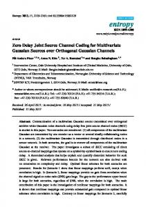
Fig. 1. Relation between the frequency axes for the noise power spectral density (in the upper left hand figure) and the signal power spectral density (in the lower right hand figure). The channel frequency axis is denoted by Fc and the source axis by Fs to distinguish between them. The straight, dashed lines in the spectral figures represent μ and θ, respectively.
Example In Figure 1 we show an example with non-white spectra and compression ratio ravg = 0.5. The spectra and the relation between the frequency axes are expressed through the bandwidth matching function. The nonlinearity of the BMF illustrates that different signal bands need different channel bandwidths to be transmitted optimally. This result can be used also if we transmit bits, indicating an optimal strategy for bit assignment to the signal frequency bands to be distributed unevenly among channel frequency bands.
4. EQUAL BANDWIDTH SYSTEMS If we transmit the source without bandwidth change (ravg = 1), there is an opportunity to use linear systems, that is transmit the source samples as continuous PAM channel symbols. However, as long as the BMF is nonlinear, OPTA cannot be reached by such a system. We may ask, can a linear system reach OPTA when the BMF is linear? The answer to this question is yes, and we will show the spectral relations for optimality. We will furthermore present the loss in using linear systems when the BMF is not linear.
Wi
Assume that we want to map the signal frequencies sequentially to the channel. The rate up to an arbitrary frequency W requires a certain channel bandwidth X, which is found by inserting Wi = 0, Wi+1 = W , Xi = 0, and Xi+1 = X in Equation 13. The equation tells us that the frequency W in the source maps to the frequency X on the channel. The function X = f (W ) will be called the bandwidth matching function (BMF).
4.1. Linear BMF Linearity of the BMF implies that X = W for W ∈ [0, Ws ] in baseband systems. Then Equation 6 simplifies to log(μθ) =
1 W
Z
W
log(SXN (F )dF, 0
(14)
where we for simplicity of notation have introduced the product spectrum1 SXN (F ) = SXX (F )SNN (F ). (15) For the relation in Equation 14 to be valid for any value of W the integrand must be constant, that is μθ = SXN (F ),
(16)
Observe that the necessary power level θ on the channel can be found from this equation if the signal and noise spectral densities are given, and we require a certain reconstruction noise level. We can derive the filtering operation necessary for preparing the signal to the channel from Equation 11: |H(F )|2 =
θ − SNN (F ) SCC (F ) = . SXX (F ) SXX (F )
(17)
This expression can be reformulated to a form compatible with a result in [2]. To simplify, we assume that we apply a zero phase FIR filter, for which case H(F ) = |H(F )|. This will be assumed for all filters in this article. The best receiver filter is assumed to be a Wiener filter as this minimizes the overall distortion. For the model where the received signal is composed of a signal filtered by the filter with frequency response H(F ) and additive, colored noise, the Wiener filter is given by: G(F ) =
SXX (F )H ∗ (F ) . |H(F )|2 SXX (F ) + SNN (F )
(18)
Using the expression in Equation 17, the filter can be expressed as „ « 1 SNN (F ) G(F ) = 1− . (19) H(F ) θ The general expression for the power spectral density of the total output noise is given by SXN (F ) SDD (F ) = . |H(F )|2 SXX (F ) + SNN (F )
(20)
For our case this reduces to SDD (F ) =
SXN (F ) . θ
(21)
Finally, if we impose the linear warping constraint from Equation 16, we find that the power spectral density of the reconstruction error is given by SDD (F ) = μ.
(22)
This is exactly the noise level we required, implying that the system with the prefilter that distributes the correct power to the channel and a corresponding Wiener filter indeed performs according to OPTA. This discussion shows that it is possible to reach OPTA for correlated sources if transmitted over channels with a noise power spectral density which is inversely proportional to the signal power spectral density. This applies only if the bandwidths of the source and the channel are the same, and the channel noise is small enough to maintain the simplifications done initially. If the channel signal power density is everywhere much larger than the noise power spectral density, we can drop the last term in Equation 17, and we obtain a whitening filter. 1 This
entity must not be confused with the cross spectral density.
4.2. Linear system performance for non-OPTA cases The transmit filter was derived under the assumption that the system acts according to OPTA. If the warping function is not linear, then this is not true, and the optimal filter will be different. The easiest way to find the optimal linear transmit filter is to minimize the reconstruction noise variance under the power constraint. The reconstruction noise variance is found by integrating Equation 20. An object function is formed by adding to this expression the channel power expression times the Lagrange multiplier. Thus we have Z W Z W SDD (F )dF + 2λ |H(F )|2 SXX (F )dF. (23) O=2 0
0
By using Gateau variation one obtains the optimal transmit filter s SNN (F ) SNN (F ) 2 − , (24) |H(F )| = λSXX (F ) SXX (F ) and the corresponding receiver Wiener filter s ! SNN (F ) 1 1− λ , G(F ) = H(F ) SXX (F )
(25)
where λ is a Lagrange multiplier which can be found from the channel power constraint as RW p √ 2 0 c SXN (F )dF λ= . (26) 2 P + σN The spectral density of the overall distortion in the received signal can be found from Equation 20 as p (27) SDD (F ) = λSXN (F ). The potential gain by using nonlinear methods over the optimal linear system (valid for ravg = 1 only) can be expressed as 12 0 RW p 1 SXN (F )dF D1 @ −4 W 0 n R o A = γ√ = , (28) p XN W D0 exp 1 log SXN (F )dF W
0
which is the squared inverse of the spectral flatness measure of the square root of the product spectrum. The case for which the product of the two spectral densities is constant renders D1 = D0 . In all other cases D1 > D0 and OPTA cannot be reached directly by linear filtering methods. 4.3. Generalization of the linear systems Even if Equation 16 is not satisfied for the case ravg = 1, we can often make this match better by reshuffling the frequency components. A practical approach to this end is to split the input signal spectrum uniformly into narrow bands by subband decomposition, and also split the channel into narrow sub-channels with the same bandwidths. If the channels are narrow enough, the spectral variations within a sub-channel could be so low that it could be considered constant. The necessary processing in the subbands is then only a constant multiplier. For a stationary signal and channel, we could furthermore reshuffle the subbands to match the sub-channels as well as possible. The optimal strategy is to pair the subband with the largest variance to
8 >
=
PM
D1 i=1 σXi σNi = “ ”1 > . > D0 M ; : QM σ σ i=1 Xi Ni
(29)
0 −1
−3 −2
0
2
4
x1
The most important conclusion from the above deliberations is that the bandwidth matching function will, in general, be nonlinear, which implies that nonlinear systems are required for optimality. This is always the case when bandwidth change is necessary or wanted, for low noise cases. In the next section we will discuss the use of nonlinear mappings in combination with the subband decomposition and OFDM transmission. Using fine decomposition and further dividing the subbands into blocks, as is most often done in image and video coding, it is found that the blocks can be well modeled by Gaussian distributions with individual variances [5]. The OFDM channels, if the bandwidths are small enough, will be essentially flat, thus allowing us to regard them as memoryless. 5.1. Bandwidth allocation We now want to study how channel bandwidth can be allocated to subbands extracted from the non-white source. Assume that we split the signal bandwidth Ws into M uniform subbands, defined in the ranges [Wi−1 , Wi ], i = 1, 2, . . . M . The idealized OFDM channel bandwidths are given by [Xj−1 , Xj ], j = 1, 2, . . . M . We can apply Equation 13 to express the relation between Xi and Xi−1 via Wi and Wi−1 , while using the approximation that the spectra are constant over the integration intervals. The ratio between the bandwidths can then be approximated to „
Xi − Xi−1 Wj − Wj−1
1
−4
5. NONLINEAR SYSTEMS
ri,j =
2
−2
As a conclusion, Equation 29 can be used to measure the closeness to OPTA for a BPAM system. OPTA is again reached when σXi σNi is independent of i because then D1 = D0 provided the decomposition is fine enough. A similar technique has been suggested in [4].
« SXX (Wj ) log μ «. „ = θ log SNN (Xi )
3
x2
the sub-channel with the lowest noise variance, then continue with the second highest signal variance and match to the second low2 est noise variance, and continue like this. Let us denote by σX i 2 and σNi the pair number i. Then the test of optimality of the new 2 σ 2 for all i. We have now obtained a system is how constant σX i Ni BPAM system [3]. The loss for this case compared to OPTA can be written in terms of the standard deviations when replacing the integrals in Equation 28 by sums:
(30)
In practice, one needs to know θ and μ before allocating the bandwidths. If a certain average bandwidth change and signal-to-noise ratio are required, one can derive these parameters from Equations 8, 7, and 9.
Fig. 2. Intertwined Archemedian spirals.
5.2. Nonlinear mappings Instead of traditional digital representation we advocate the application of Kotelnikov-Shannon mappings, which implies that the analog samples are mapped to spaces of different dimensions, either by combining samples to fewer components or splitting samples into more components. Oversampling, which is similar to repetition codes, is a linear expansion method, while lowpass-filtering followed by downsampling is a linear method for signal compression. Both of these are highly nonoptimal. It is outside the scope to discuss in detail different nonlinear mappings. We will just mention the Archemedian spiral as a possible method for both 2:1 and 1:2 mappings as shown in Figure 2. Used as a 2:1 mapping, an original two-dimensional signal vector (x1 , x2 ) is shown in Figure 2 as a filled circle. We approximate this vector to the closest point on one of the spiral arms, which is shown as a filled square. The signal component can be transmitted as a continuous PAM symbol with a value given by the distance from this point to the origin along the spiral. If the approximation point is on the solid line, the transmitted symbol will be positive, if it is on the dashed curve, the channel symbol will be negative. When the signal experiences channel noise, its value is changed, and when measuring the received value along the spiral, the vector indicated by the filled diamond results. The approximation and channel noise are close to orthogonal provided the spiral is dense and the channel noise is small. Robustness towards channel error is a result of the analog nature of the channel symbol. The noise will move it along the spiral, so moderate noise components only change the two signal components slightly. Used as a 1:2 mapping, the original can be inserted into the figure by measuring its amplitude along the spiral, now given by the diamond. The coordinates x1 and x2 are transmitted independently or as QAM symbols. Channel noise will move the vector off the circle. The decoder knows that the original transmitted signal resided on the spiral, and will therefore use as the 2-D estimate the closest point on the spiral (square). The decoded signal is then given by distance from the square to the origin. The spiral density has to be matched to the input signal variance and the channel noise. This will mandate a need for several mappings of each dimension change in practical JSCC systems. In a companion paper [6] the performances of these mappings are analyzed. They perform close to the best known mappings for these dimension changes. Other mappings can be found in [7].
5.3. Some system details Equation 30 tells us that we may need arbitrary bandwidth changes, while in the practical world only rational ratios are implementable as we need to combine a certain number of source parameters and map them onto a number of channel samples. With a set of possible mappings, the optimal rate change has to be approximated to one of the available values. Then to obtain a given overall rate, the first problem we face is to balance the sum of rates after quantizing each to them. One can set up several smart algorithms to approximate the correct rate. If very accurate rates are required, the mapping allocation may have to be done iteratively. With the inaccurate mappings the performance will also suffer. We can maximize the practical performance in several ways to counteract the loss by using nonoptimal mappings. Once the signal is split into subbands one may choose to transmit any of the subbands in any of the sub-channels, and thus try to get close to an available value of r. The second measure we resort to is a reallocation of power. From the ideal theory the channel power is allocated according to the water filling principle. However with nonoptimal rate, this is no longer optimal. We experienced the same for the linear case when it was no longer optimal (compare Equations 17 and 24). We will not derive the optimal power reallocation in this paper. Now assume the signal is split ideally into M subbands of bandwidth ΔF = Ws /M , where ΔF is small enough to produce close to white subbands, and we form blocks of N samples in each band. For each block the RMS value is calculated and used as an estimate of the local standard deviation. Choose as the OFDM channel bandwidths a fraction of the source bandwidth given by ΔF/N = Ws /(M N ). If the channel is stationary, it suffices to estimate the noise variance in each of the sub-channels. From Equation 30 the necessary dimension changes can be found when using the obtained variances instead of the spectral densities. The available mappings are constrained to dimension changes r = k/l, where k and l are relatively prime integers. As an example, let us be practical and assume that the following mappings are available: r = k/l = [2, 1, 2/3, 1/2, 1/4, 0]. Then by choosing source block-lengths N = 12, the different mappings will produce [24, 12, 8, 6, 4, 3, 0] channel samples. After matching the sources to appropriate channels and adjusting the rates to an overall bandwidth relation, the power is reallocated for optimal performance. This concludes the practical allocation procedure, and the actual mappings and transmissions can start. A similar system for transmitting images over AWGN channels has been developed in [8]. 6. CONCLUSION In this paper we have discussed the potential of joint source-channel coding (or joint source coding and modulation) for colored Gaussian sources and Gaussian channels with memory. We have presented the performance limits in terms of OPTA when the channel power is constrained, and introduced a bandwidth matching function which tells how to allocate channel bandwidth to the different frequency regions of a non-white source signal. The bandwidth matching function has first been used to derive optimal linear systems. Then we have seen how this also can be a tool for finding optimal resource allocations between signal subbands and OFDM channels. Finally, Kotelnikov-Shannon mappings were briefly discussed to indicate the potential of constructing nonlinear dimen-
sion changing mappings. Traditional signal transmission systems use an intermediate bit representation derived by digital signal compression followed by complicated FEC and adapted channel access methods. Such systems always experience the water fall effect when the channel deteriorates below its design operating point. This is due to what Shannon calls the threshold effect [9], and cannot be avoided in systems using bit representations. With direct mappings, the threshold effect is present for dimension increase, but not for mappings where the dimension is decreased. In practical systems many different mappings will be applied dynamically, and thus the influence of the threshold effect will be more limited. This also indicates that for increasing the robustness, one should try to avoid dimension expansion. The mechanism for that is firstly through the combination of source and channel samples, and secondly through power compensation. Whereas the first remedy does not influence optimality, the second would. One would also try to avoid dimension increasing mappings because they perform further away from OPTA. The most promising applications are for image and video transmission due to the fairly small dynamic range present in the signal parameters. Then robust systems can be devised for channels with rather limited CSNRs. Future work will include full simulation of image transmission over realistic channels. 7. REFERENCES [1] T. Berger, Rate Distortion Theory, Prentice-Hall, Inc, Englewood Cliffs, New Jersey, 1971. [2] Are Hjørungnes, Optimal Bit and Power Constrained Filter Banks, Ph.D. thesis, Norwegian University of Science and Technology, 2000. [3] Kyong-Hwa Lee and Daniel P. Petersen, “Optimal linear coding for vector channels,” IEEE Trans. Commun., vol. COM24, no. 12, pp. 1283–1290, Dec. 1976. [4] V. Kafedziski, “Linear coding of continuous-amplitude sources over siso and mimo fir channels with ergodic coefficients,” ITW2003, 2003. [5] John M. Lervik and Tor A. Ramstad, “Optimality of multiple entropy coder systems for nonstationary sources modeled by a mixture distribution,” in Proc. Int. Conf. on Acoustics, Speech, and Signal Proc. (ICASSP), Atlanta, GA, USA, May 1996, IEEE, vol. 4, pp. 875–878. [6] P. A. Floor and T. A. Ramstad, “Noise analysis for dimension expanding mappings in source-channel coding,” SPAWC’06, 2006. [7] Arild Fuldseth, Robust Subband Video Compression for Noisy Channels with Multilevel Signaling, Ph.D. thesis, Norwegian University of Science and Technology, June 1997. [8] H. Coward, Joint Source-Channel Coding: Development of Methods and Utilization in Image Communications, Ph.D. thesis, Norwegian University of Science and Technology, 2001. [9] Claude E. Shannon, “A mathematical theory of communication,” Bell Syst. Tech. J., vol. 27, pp. 379–423 and 623–656, 1948.