University of Florida, Gainesville, FL 32611. 2Department of Earth ... is among the best distributions proposed to fit non-Gaussian sea clutter data. Using diffusive ...
On modeling sea clutter by diffusive models Jing Hu1 ,Wen-wen Tung2, Jianbo Gao1 , Robert S. Lynch3, and Genshe Chen4 1 Department of Electrical and Computer Engineering University of Florida, Gainesville, FL 32611 2 Department of Earth & Atmospheric Sciences, Purdue University, West Lafayette, IN 47907 3 Signal Processing Branch Naval Undersea Warfare Center, Newport, RI 02841 4 DCM Research Resources LLC Germantown, MD 20874 ABSTRACT Sea clutter, the radar backscatter from the ocean surface, has been observed to be highly non-Gaussian. K distribution is among the best distributions proposed to fit non-Gaussian sea clutter data. Using diffusive models, K distributed sea clutter can be casted as a Gaussian speckle, with a de-correlation time of 0.1 s, modulated by a Gamma distribution, with a de-correlation time of about 1 s, characterizing the large scale structures of the sea surface. Our analyses of large amounts of real sea clutter data suggest that between the time scales for the Gaussian speckle and large scale structures on the sea surface to de-correlate, sea clutter can be characterized as multifractal 1/f processes. This is the feature that is not captured by diffusive models and underlies why K distribution cannot fit real sea clutter data sufficiently well. We surmise that by combining K distribution and associated diffusive models with multifractal formalism, the many different physical processes underlying sea clutter can be more comprehensively characterized.
1
INTRODUCTION
Sea clutter, the radar backscatter from the ocean surface, is highly complicated and non-stationary [1], due to multipath propagation of the radar returns and multiscale interactions at the air-sea interface. The latter involve ocean sprays, capillary waves, wind waves, and swells, all affecting the roughness of the sea surface. Accurate modeling of sea clutter and rough sea surface is an important problem in radar signal processing and applications, as it will facilitate robust detection of low observable targets within sea clutter, which has significant importance to coastal security, navigation safety and environmental monitoring.
Signal Processing, Sensor Fusion, and Target Recognition XVII, edited by Ivan Kadar Proc. of SPIE Vol. 6968, 69681F, (2008) · 0277-786X/08/$18 · doi: 10.1117/12.777202
Proc. of SPIE Vol. 6968 69681F-1 2008 SPIE Digital Library -- Subscriber Archive Copy
It is well-known that sea clutter data are often highly non-Gaussian. There has been much effort to fit various distributions to the observed amplitude data of sea clutter. Among the various distributions proposed to fit non-Gaussian sea clutter data, including Weibull, log-normal, K, and compound-Gaussian distributions [2–6], K distribution is considered the best. Originally, it was formulated in terms of coherent scattering and statistics of fluctuating population of scatters [7]. Recently, using random walk and diffusion models, Tough and Ward [8] have derived elegant stochastic differential equations and associated Fokker-Planck equations, and re-casted the K distribution as a Gaussian speckle process with its local power modulated by a gamma distribution. The reformulation interprets sea clutter as Gaussian speckle over short periods, with de-correlation time on the order 0.1 s, corresponding to transit of small scale sea surface features through the microwave wavelength. The modulation represented by the gamma variate is considered to be associated with the large scale structure of the sea surface, partially resolved by the high resolution radar; its de-correlation time is typically of the order of seconds or more. Although the reformulation is theoretically very attractive, Tough and Ward [8] have cautioned that the relatively simple dynamics captured by diffusive models may not be sufficiently flexible to mimic the correlation properties of sea clutter realistically. To quantitatively appreciate the effectiveness and limitations of diffusive models, in this paper, we first examine the goodness-of-fit of real sea clutter data using the K distribution. Then we carry out multifractal analysis of sea clutter, to identify important time scales and the detailed correlation structure of sea clutter. The remainder of the paper is organized as follows. In Sec. 2, we briefly describe sea clutter data. In Sec. 3, we examine how well K distribution fits real sea clutter data. In Sec. 4, we carry out structure-function–based multifractal analysis of sea clutter. Finally, in Sec. 5, we make a few concluding remarks.
2 SEA CLUTTER DATA Fourteen sea clutter datasets were obtained from a website maintained by Professor Simon Haykin: http://soma.ece.mcmaster.ca/ipix/dartmouth/datasets.html. The measurement was made using the McMaster IPIX radar at Dartmouth, Nova Scotia, Canada. The radar was mounted in a fixed position on land 25-30 m above sea level, with an operating (carrier) frequency of 9.39 GHz (and hence a wavelength of about 3 cm). It was operated at low grazing angles, with the antenna dwelling in a fixed direction, illuminating a patch of ocean surface. The mea-
Proc. of SPIE Vol. 6968 69681F-2
h : Antenna height φ : Grazing angle : Range (distance from the radar) Ri B1 ~ B14 : Range bins Target
φ
h B1 B2
⋅⋅⋅
B
i−1
o
B
i
B
i+1
⋅⋅⋅
B14
(Secondary) (Primary)(Secondary)
R
i
Figure 1: A schematic showing how the sea clutter data were collected. surements were performed with the wave height in the ocean varying from 0.8 to 3.8 m (with peak heights up to 5.5 m) and the wind conditions varying from still to 60 km/hr (with gusts up to 90 km/hr). For each measurement, 14 areas, called antenna footprints or range bins, were scanned. Their centers are depicted as B 1 , B2 , · · · , B14 in Fig. 1. The distance between two adjacent range bins was 15 m. One or a few range bins (say, B i−1 , Bi and Bi+1 ) hit a target, which was a spherical block of styrofoam of diameter 1 m wrapped with wire mesh. The locations of the three targets were specified by their azimuthal angle and distance to the radar. They were (128 0, 2660 m), (130 0, 5525 m), and (1700, 2655 m), respectively. The range bin where the target is strongest is labeled as the primary target bin. Due to drift of the target, bins adjacent to the primary target bin may also have hit the target. They are called secondary target bins. For each range bin, there were 2 17 complex numbers, sampled with a frequency of 1000 Hz.
3 GOODNESS-OF-FIT OF THE K DISTRIBUTION As mentioned earlier, K distribution has been considered the best distribution proposed to fit sea clutter data. K distribution is described by the following probability density function, �ν � �� �� √ 2ν 2ν 2ν x Kν−1 x , x≥0 f (x) = √ µΓ(ν)2ν−1 µ µ
(1)
where µ is half of the second moment, ν − 1 is the order of the modified Bessel function of the third kind, K ν−1 , and Γ(ν) is the usual gamma function. We have found that fitting of real sea clutter data using K distribution is not excellent. Two typical examples are shown in Fig. 2(a,b). Furthermore, we have found that the key parameters involved in the K distribution are not effective for distinguishing sea clutter data with targets from those without targets.
Proc. of SPIE Vol. 6968 69681F-3
0.8
0.8
(b)
0.7
0.7
0.6
0.6
0.5
0.5
PDF
PDF
(a)
0.4
0.3
0.3 Data K distribution fit
0.2 0.1 0
0.4
0.5
1 x
0.2
1.5
0.1 0
2
Data K distribution fit 0.5
1 x
1.5
2
Figure 2: Representative results of using K distribution to fit the amplitude data of sea clutter. (a) is for the sea clutter data without target, while (b) is for the data with target. Circles and solid lines denote the raw and fitted probability density functions (PDFs), respectively.
4 STRUCTURE-FUNCTION–BASED MULTIFRACTAL ANALYSIS OF SEA CLUTTER One of the simplest multiscale analyses is the structure-function based multifractal formulation [1, 9] It is especially convenient for the study of the ubiquitous 1/f noise, a type of spatial or temporal variations whose power-spectraldensity (PSD) decays in a power-law manner. For examples of 1/f processes, we refer to our recent book [1], especially Chapter 8. To better understand the structure-function based multifractal formulation, let us start from a brief review of random walk model that forms the building blocks of the Tough and Ward’s model [8]. In that model, the electric field returned from N coherently illuminated scatterers is written as a two-dimensional vector sum of the contributions a k from the individual scatterers E=
N
∑ ak
(2)
k=1
and is thought of as the resultant of a random walk of N steps. In their model, a k are assumed to be independent, isotropically distributed and statistically identical. As we shall see momentarily, such an assumption fixes the Hurst parameter to be 1/2, and therefore, has to be discarded. It is now straightforward to understand how multifractal analysis of sea clutter should proceed. The key is to
Proc. of SPIE Vol. 6968 69681F-4
interpret the sea clutter data, y(n), n = 1, · · ·, as a “random walk” process, and examine whether the following scalinglaw holds or not, F (q) (N) = �|y(i + N) − y(i)|q�1/q ∼ N H(q) ,
(3)
where H(q) is a function of real value q, and the average is taken over all possible pairs of (y(i + N), y(i)). Large positive values of q emphasizes large differences in y(n). Large negative values of q emphasizes small differences in y(n). When the scaling laws described by Eq. (3) hold, the process under investigation is said to be a fractal process. Furthermore, if H(q) is not a constant of q, the process is a multifractal; otherwise, it is a monofractal. The case of q = 2 is of special interest. It characterizes the correlation structure of the data set: depending on whether H(2) is smaller than, equal to, or larger than 1/2, the process is said to have anti-persistent, short-range, or persistent longrange correlations [1, 9]. In fact, when Eq. (3) holds and H(2) �= 1/2, the autocorrelation for the “increment” process, defined as x(i) = y(i + 1) − y(i), decays as a power-law, r(k) ∼ k 2H(2)−2 , as k → ∞, while the PSD for y(n), n = 1, · · · is Ey ( f ) ∼ 1/ f 2H(2)+1 . H(2) is often called the Hurst parameter, and simply denoted as H. To better appreciate the meaning of the Hurst parameter, let us focus on the increment process x(i). We construct a new time series x(m) = {x(t)(m) : t = 1, 2, 3, . . .}, m = 1, 2, 3, . . . , obtained by averaging the original series x over nonoverlapping blocks of size m, x(t)(m) = (x(tm − m + 1)+ · · · + x(tm))/m, t ≥ 1 .
(4)
When the scaling law of Eq. (3) with q = 2 holds, one can readily prove that the variance of x (m) satisfies var(x(m) ) = σ2 m2H−2
(5)
Using Eq. (5), we can conveniently examine the effectiveness of smoothing when H varies. If H = 1/2, for the variance to drop to 10 −2 of its original value, m = 100. When H = 3/4, we have to choose m = 10000, in order to let the variance drop to 10 −2 of its original value. On the other hand, when H = 1/4, then choosing m = 10 4/3 ≈ 17 is sufficient to make the variance to be 10 −2 of its original value. These simple numerical values should give one a concrete understanding of the meaning of persistent and anti-persistent long range correlations.
Proc. of SPIE Vol. 6968 69681F-5
0.4
1 0.5
(a)
0.35
−1 −1.5
Bins With Targets
0.25 0.2 0.15
−2
0.1
−2.5 −3 0
Primary Target Bin
0.3
−0.5 H(2)
log2 F(2) (N)
0
(b)
2
4
6
8 10 12 14 16 log N
0.05 0
2
2
4
6 8 10 12 14 Bin Number
Figure 3: (a) log2 F (2) (N) vs. log2 N for the 14 range bins; (b) The H(2) values for the 14 range bins. Open circles denote bins with target, while * denote bins without targets. To find out whether Eq. (3) holds or not for sea clutter data, we have analyzed all the data available to us. Fig. 3 shows a representative result for q = 2. In the time scale range of 30 ms to about 1 s (which corresponds to N = 5 to 10), we observe three interesting features: (i) H(2) < 1/2, for both sea clutter data with and without targets. Therefore, the “increment” processes of sea clutter always have anti-persistent long-range correlations. Note such a property cannot be readily described by simple diffusive models. (ii) H(2) is much larger when the range bins hit a target, therefore, it can be used to effectively detect targets within sea clutter. (iii) When a range bin hit a target, H(2) is close to 1/3. This reminds one of the famous Kolmogorov’s energy spectrum for fully developed turbulence: E( f ) ∼ f
−5/3
= f −(2× 3 +1) 1
with H = 1/3. This suggests that wave-turbulence interaction is an important element of sea clutter dynamics when there is a target. To find out whether sea clutter data are multifractals, we have examined other values of q. Figs. 4(a,b)show representative log2 F (q) (m) vs. log2 m curves for a number of q values for two sea clutter data, one is without the target, the other with the target. The variation of H(q) vs. q for the 14 range bins data of one measurement is shown in Fig. 5. We observe that the sea clutter data appear to be multifractal, especially for data with the target. The effectiveness of H(2) for distinguishing data with and without the target stimulates us to examine if H(q) values for other q may have similar power. This turns out to be generically true, as shown in Fig. 6 for three examples of H(q) vs. q. Therefore, sea clutter data are multifractals.
Proc. of SPIE Vol. 6968 69681F-6
3
3
2 (b)
(a) (m)
1 (q)
1
2
log F
log2 F(q) (m)
2
0
0 −1 −2 −3
−1
−4 −2 0
2
4
6
8 10 12 14 16 log2 m
−5 0
2
4
6
8 10 12 14 16 log m 2
Figure 4: Representative log 2 F (q) (m) vs. log2 m curves for a number of q values for the sea clutter data (a) without and (b) with target. Curves from bottom to top correspond to q = 1, 2, · · · , 6. Let us now focus on H(2) and critically examine if a robust detector for detecting targets within sea clutter can be developed based on H(2). We have systematically studied 392 time series of the sea clutter data measured under various sea and weather conditions. To better appreciate the detection performance, we have first only focused on bins with primary targets, but omitted those with secondary targets, since sometimes it is hard to determine whether a bin with secondary target really hits a target or not. After omitting the range bin data with secondary targets, the frequencies for the H(2) parameter under the two hypotheses (the bins without targets and those with primary targets) for HH and VV datasets are shown in Figs. 7(a,b), respectively. We observe that the frequencies completely separate for the HH datasets. The accuracy for the VV datasets is also very good, except for two measurements. Interestingly, those two measurements correspond to the two HH measurements with the two smallest H(2) values. We emphasize that the accuracy of target detection within sea clutter critically depends on the time scale range of 30 ms to about 1 s we identified. On time scales smaller than 30 ms, we have found that sea clutter data are actually quite smooth; on time scales longer than 1 sec, sea clutter data are very irregular.
5
CONCLUDING REMARKS
To better appreciate the effectiveness and limitations of diffusive models, which underlie the physical foundations for the K distribution, in this paper, we have examined the goodness-of-fit of real sea clutter data using the K distribution.
Proc. of SPIE Vol. 6968 69681F-7
0.4 0.35 0.3
H(q)
0.25 0.2 0.15 0.1 0.05 0 0
1
2
3
4
5
6
q
Figure 5: The variation of H(q) vs. q curves for the 14 range bins. 0.4
0.4
H(q)
0.4 q=1
q = 0.1
q=3
0.3
0.3
0.3
0.2
0.2
0.2
0.1
0.1
0.1
0 0
5 10 Bin Number
0 0
15
5 10 Bin Number
15
0 0
5 10 Bin Number
15
Figure 6: H(q), q = 0.1, 1, 3 for the 14 range bins. Circles represent range bins with target. We have found that the fitting is not as good as one would desire. More seriously, the parameters derived from the K distribution fit cannot be used to effectively detect low observable targets within sea clutter. The shortcomings of the K distribution have motivated us to carry out multifractal analysis of sea clutter. We have successfully identified an interesting time scale range of 30 ms to about 1 s. Within this time scale range, we have found that both sea clutter data with and without targets can be characterized as multifractal 1/f type processes with anti-persistent long range correlation. Furthermore, the H(q) spectrum, which includes the Hurst parameter as a special case, can be used to very effectively detect targets within sea clutter. As we noted earlier, the diffusive models of Tough and Ward [8] also prescribe two time scales. One is on the order
Proc. of SPIE Vol. 6968 69681F-8
18 16
(a)
no targets primary targets
14 Frequency
12 10 8 6 4 2 0
0
0.1
0.2
0.3
0.4
0.5
30 (b)
no targets primary targets
25
Frequency
20 15 10 5 0 0
0.05
0.1
0.15
0.2
0.25
0.3
0.35
H(2)
Figure 7: The frequencies of the bins without targets and the bins with primary targets for (a) HH and (b) VV datasets. of 0.1 s, characterizing de-correlation time of Gaussian speckle. The other is about 1 s, characterizing de-correlation time of large scale structure of the sea surface. Our multifractal analysis suggests that between these two time scales, sea clutter data can be readily characterized as multifractal 1/f processes. This is the major feature that is not captured by diffusive models and underlies why K distribution cannot fit real sea clutter data very well. We believe that by combining K distribution and associated diffusive models with multifractal formalism, sea clutter should be better modeled, in the sense that physical processes occurring on vastly differing time scales can be more comprehensively characterized.
Proc. of SPIE Vol. 6968 69681F-9
References [1] J.B. Gao, Y.H. Cao, W.W. Tung, and J. Hu, Multiscale Analysis of Complex Time Series — Integration of Chaos and Random Fractal Theory, and Beyond, Wiley, August, 2007. [2] F.A. Fay, J. Clarke, and R. S. Peters, “Weibull distribution applied to sea-clutter”, Proc. IEE Conf. Radar’77, London, U.K., pp. 101-103, 1977. [3] F.E. Nathanson, Radar design principles (McGraw Hill), pp. 254-256, 1969. [4] E. Jakeman and P.N. Pusey, “A model for non Rayleigh sea echo”, IEEE Trans Antennas & Propagation, 24, 806-814, 1976. [5] S. Sayama and M. Sekine, “Log-normal, log-Weibull and K-distributed sea clutter”, IEICE Trans. Commun. E85-B, 1375-1381, 2002. [6] F. Gini, A. Farina, and M. Montanari, “Vector subspace detection in compound-Gaussian clutter, Part II: performance analysis”, IEEE Transactions on Aerospace and Electronic Systems 38, 1312-1323, 2002. [7] E. Jakeman and P.N. Pusey, Significance of k-distributions in scattering experiments, Phys. Rev. Lett. 40, 546 (1978). [8] R.J.A. Tough and K.D. Ward, Diffusive and related models of some properties of sea clutter, J Phys-Condens Mat 14, 7737-7748 (2002). [9] J.B. Gao, J. Hu, W.W. Tung, Y.H. Cao, N. Sarshar, V. P. Roychowdhury, Assessment of long range correlation in time series: How to avoid pitfalls. Phys. Rev. E 73, 016117 (2006).
Proc. of SPIE Vol. 6968 69681F-10