On parallelization of a spatially-explicit structured ecological model for integrated ecosystem simulation
Dali Wang Department of Computer Science University of Tennessee, Knoxville, TN 37996-3450, USA.
Michael W. Berry Department of Computer Science University of Tennessee, Knoxville, TN 37996-3450, USA.
Louis J. Gross Departments of Ecology and Evolutionary Biology and Mathematics University of Tennessee, Knoxville, TN 37996, USA.
1
Summary: Spatially explicit landscape population models are widely used to analyze the dynamics of an ecological species over a realistic landscape. These models may be data intensive applications when they include the age and size structure of the species in conjunction with spatial information coming from a geographic information system (GIS). We report on parallelization of a spatially explicit landscape model (PALFISH), in a component-based simulation framework, utilizing different parallel architectures. A multithreaded programming language (Pthread) is used to deliver high scalability on a symmetric multiprocessor (SMP), and a message-passing library is deployed for parallel implementation on both an SMP and a commodity cluster. The PALFISH model delivers essentially identical results as a sequential version but with high scalability: yielding a speedup factor of 12 as the runtime is reduced from 35 hours (sequential ALFISH) to 2.5 hours on a 14-processor SMP. Hardware performance data were collected to better characterize the parallel execution of the model on the different architectures. This is the first documentation of a high performance application in natural resource management that uses different parallel computing libraries and platforms. Due to the diverse needs for computationally intensive multimodels in scientific applications, our conclusions arising from a practical application which brings the software component paradigm to high-performance scientific computing, can provide guidance for appropriate parallelization approaches incorporating multiple temporal and spatial scales. Running title:
Parallelization of an ecological model
Authors: Dr. Dali Wang (corresponding author) Department of Computer Science University of Tennessee, Knoxville, TN 37996-3450, USA. Phone: (865) 974-2773 Fax: (865) 974-3067 Email:
[email protected] Dr. Michael W. Berry Department of Computer Science The University of Tennessee, Knoxville, TN 37996-3450, USA. Phone: (865) 974-3838 Fax: (865) 974-4404 Email:
[email protected] Dr. Louis J. Gross Departments of Ecology and Evolutionary Biology and Mathematics University of Tennessee Knoxville, TN 37996, USA. Phone: (865) 974-4295 Fax: (865) 974-3067 E-mail:
[email protected]
2
1
Introduction
Ecosystem modeling presents a variety of challenges. Traditional ecosystem modeling is sequential and not spatially explicit. Researchers typically analyze model solutions mathematically and then compare them to abundance estimates from field or lab observations. Although highly influential in ecological theory, the aggregated form of the underlying differential equation models is particularly difficult to relate to observational biology. Ecosystem dynamics has a significant spatial component, involving the distribution of species habitats, and proximity of ecological populations to human activities (i.e., effects of harvesting). Therefore, recent emphasis has been on spatially-explicit, integrated ecosystem models. The main purpose of ecosystem modeling is to simulate the functioning of an ecosystem to enhance understanding and ensure appropriate human management. Due to the inherent multi-scale nature of ecosystems, ecological multimodeling is one of the natural choices for integrated simulation [3]. In an ecological multimodeling framework, different ecological models/approaches are used for organisms at different hierarchical levels. These models involve complex interactions between some or all of an ecosystem’s trophic layers (feeding levels), resulting in models that link multiple components based on different mathematical approaches. Compared to traditional approaches in engineering and weather/climate systems, ecosystem components function at a diversity of temporal scales. Moreover, ecosystem can be intensively influenced by human activities. Hence ecological models need to incorporate human management options, which in turn determine the structure of an ecosystem simulation system, such as interface design, parameter calibrations, uncertainty /sensitivity analysis, etc. A component-based simulation framework is a favorable choice for multiscale ecosystem simulation, which requires dedicated coupling to support flexible data communication/exchange between components, computational parallelism and on-demand dynamic load balancing [13]. Thus ecological models and human activities need to be linked and modeled (parallel to each other) as components in an ecosystem simulation
3
package. Integrated ecosystem simulations therefore require more flexible software design than many multi-component simulations in computational fluid dynamics (CFD). In those CFD simulations, the highly-coupled Navier-Stokes equations and other equations are solved simultaneously by sophisticated numerical algorithms. Sequential data flow is typically preferred and enforced to simplify the procedure of data exchange between components, automatic mesh generations and dynamic loading balance (if parallel computation is required) between individual components (see www.casr.uiuc.edu for example). Recently, grid computing has become a popular approach for integrated ecosystem simulation [9]. In a grid computing environment, ecosystem models need to be implemented on heterogeneous platforms (cluster, symmetric multiprocessor (SMP)) using different computational modes (i.e., multithreaded or multiprocess mode). In this paper, we report on our experience and lessons learned from parallelizing a spatially-explicit structured ecological model on two high-performance computational platforms (i.e. a cluster and a symmetric multi-processor (SMP)) using POSIX threads (Pthreads) and message-passing interface (MPI). Spatially-explicit structured ecological models (SEM) are becoming more commonly used in ecological modeling, in part due to the availability of new spatial data sets. Those models average certain population characteristics and attempt to simulate changes in these characteristics for the whole population. In general, structured ecological models use a set of structured classes (age, size, physiological status) to model a population. The range used for each structured class, along with the model’s time step, influences the model’s parameter values and affects the transition rates between classes. In an SEM, all states of the population, at each location, can be well defined and the spatially-explicit patterns which arise can be coupled with data from remote sensing and geographic information systems.1 Increasing computational capabilities now make it feasible to break down populations and communities into discrete species (or classes), and to develop a series of linked SEMs which take into account details of the size, age, and physiological state structure of each 1 Geographic Information Systems (GIS) technology is used extensively in ecosystem modeling to visualize, analyze, and model data for management and problem solving. However, a GIS is generally inefficient for problems involving dynamic modeling of populations and is typically not designed for high performance computation.
4
species (or class). Such an SEM can include 100-1000 state variables within a single localized landscape cell, so that high performance computation is required [10]. In this paper, we focus on several important issues related to the parallelization of spatially-explicit structured landscape ecological models in the context of integrated ecosystem modeling, covering computational model design, landscape partitioning, dynamic load balancing, synchronization, and performance analysis as well as implementation strategies for different computer architectures. Our observations can serve as general guidelines for the efficient parallelization of spatially-explicit structured ecological models and integration of multimodels on high performance computers. As with many multi-component applications involving inter-linked processes operating on multiple scales, our results and experience, which come from a practical application of bring the software component paradigm to high-performance scientific computing, can be applicable to many research problems in hydrology, micrometeorology, and climate/weather modeling. An example is hydrologic models with daily, yearly, and decade time scales which links to vegetation changes and associated soil dynamics.
2
Computational Environments and Software
The two computational platforms used in this research are components of the Scalable Intercampus Research Grid (or SInRG, icl.cs.utk.edu/sinrg) at the University of Tennessee, Knoxville. One is a Sun Microsystem Enterprise 4500 symmetric multiprocessor (SMP) configured with 14 400MHz Sun Ultra Sparc II processors (see Fig. 1). Each processor has a 16KB instruction cache and a 16KB data cache on chip, plus an 8MB external cache for high performance computation. The entire system has 10 GB main memory and is connected via a 3.2 GB/s system bus. The total storage capacity of this system is 1.5 Terabytes. The other component is a 16-node Sun Microsystem cluster. Each node has dual 450MHz Sun Ultra Sparc II processors. Each processor has a 16KB instruction cache and a 16KB data cache on chip, plus a 4MB external cache for high performance computation.
5
Figure 1: Schematic of the Sun Enterprise 4500 SMP
Each node has 512MB main memory and a 30GB local hard disk. All nodes are connected via a 1Gb/s Ethernet network with dedicated switches. The general architecture of the cluster is depicted in Fig. 2. An implementation of the MPI standard library, LAM-MPI
Figure 2: Schematic of the Sun cluster
(www.lammpi.org), was selected to support message-passing in the parallel implementations. An implementation of the IEEE POSIX 1003.1c standard (1995) POSIX threads (Pthreads)[12] was selected to support the multithreaded programming on the SMP.
3
General Computational Model
In the context of integrated simulation for ecological multimodels, a master-slave model was chosen as the general computational model. Here, the master process/thread collects partial computational results from all slave processes/threads, referred to as computational processes/threads, and stores assembled results on disk. There are some advantages 6
associated with this computational model. From a performance standpoint, the master process/thread separates the time-consuming I/O operations from the much faster computational phases, which increases the efficiency of data access during the simulation. More importantly, the master process/thread provides a uniform, transparent interface for integration with other ecological models [11]. The particular model emphasized in this study is one component of a multimodel, ATLSS (Across Trophic Level System Simulation), which was developed to assist South Florida hydrological management in Everglades restoration planning.
3.1
Landscape Partitioning
One-dimensional (1D) partitioning (e.g., a row-wise, block-striped) can be a convenient and efficient approach to decomposing the landscape in structured ecological models. First, such models are generally used for regional ecosystem simulation, in which the computational domain (landscape) is not massive. Unlike individual-based ecological models, structured ecological models are aggregated population models developed for a given species. In addition, the size of a single landscape cell, as determined based upon the underlying behavior of the species of concern, cannot be too small. Thus the computational domain (problem size) of this kind of model is limited. Second, spatially-explicit structured ecological models are generally data intensive applications, so that even simple 1D static partitioning yields significant communication overheads. Communication overheads become even more burdensome with two-dimensional partitioning. In the context of the PALFISH (Parallel Across Landscape Fish) model investigated here, external forces (such as water depth, which is controlled by human activities) determine fish behaviors and dramatically change the computational workload associated with different landscape regions, therefore, 1D partitioning is implemented. See [8] for more details on one-dimensional static partitioning of a landscape.
7
3.2
Dynamic Load Balancing
A dynamic load balancing technique was implemented to better distribute the computational workload2 among different processors. In addition, an imbalance-tolerance threshold was set to limit the extra communication overhead introduced by dynamic balancing of computational workload during the simulation. Generally, the procedure for computational workload balancing consists of the following operations: 1. Each computational processor determines its workload at each step by recording the time used for computation; 2. The master processor compares all workloads on computational processors and determines which landscape rows are needed to be exchanged between processors, if an imbalance is found to be larger than the predefined imbalance-tolerance; 3. In the MPI implementation, the information on new partitioning boundaries is passed to computational processors along with the associated data within the exchanged rows. In the Pthread implementation, only the information on new boundaries is passed to computational threads.
3.3
Synchronization
Synchronizations are inevitable in parallel implementations. Using MPI, synchronizations can be easily achieved by deploying blocking communication primitives (i.e., MPI Send, MPI Recv and MPI Sendrecv). In addition, MPI Barrier can also guarantee explicit synchronizations during simulation. POSIX implements three synchronization variables mutex, semaphore, condition variables and the function pthread join to provide synchronization functionality. There is no similar barrier function to MPI barrier. Therefore, a thread barrier function was implemented (see Fig. 3). 2 Computational
time was used as the measure of computational workload on each processor.
8
typedef struct barrier tag { pthread mutex t mutex pthread cond t cw int valid int threshold int counter int cycle } barrier t
/* /* /* /* /* /*
control access to barrier */ wait for barrier */ set when valid */ number of threads required */ current number of threads */ alternative wait cycles */
Figure 3: Data structure for thread barrier function in POSIX
4
Across Landscape Fish Population Model
The Across Landscape Fish Population (ALFISH) model[4, 7] is an example of a complicated spatially-explicit structured ecological model, and is one component of the Across Trophic Level System Simulation (ATLSS, www.atlss.org), an ecological multimodel designed to assess the effects on key biota of alternative water management plans for the regulation of water flow across the Everglades landscape[3]. The ALFISH model includes two main subgroups (small planktivorous fish and large piscivirous fish), structured by size. One objective of ALFISH parallelization is to speedup the ALFISH execution for its practical use within ATLSS by allowing real-time data generation and information sharing between multiple ATLSS models. For example, ALFISH interacts with various wading bird models within ATLSS. Speedup permits broader use of ALFISH in integrated regional ecosystem modeling [11], assists future scenario evaluations and increases accessibility for natural resource managers at various South Florida agencies, through a grid service module [9].
4.1
ALFISH Model Structure
The study area for ALFISH contains 26 regions as determined by the South Florida Water Management Model[6]. The total area of the Everglades modeled in ALFISH contains approximately 111,000 landscape cells, with each cell 500m on a side. Each landscape cell has two basic types of area: marsh and pond. In the marsh area of each cell, there is an elevation distribution based upon a hypsograph[2]. This hypsograph is used to determine
9
the fraction of the marsh area that is still under water at a given water depth. A pond refers to permanently wet areas of small size, such as alligator holes, which are a maximum of 50 m2 or 0.02% of the cell. In ALFISH, spatial and temporal fluctuations in fish populations are driven by a number of factors, especially the water level. Fluctuations in water depth affect all aspects of the trophic structure in the Everglades. The fish population simulated by ALFISH is size-structured and is divided into two functional groups: small and large fishes. Both of these groups appear in each of the marsh and pond areas. Each functional group in each area is further divided into several age groups (40 and 25 respectively), and each age group has 6 size groups. The fish population in each cell is summarized by the total fish density (biomass) within that cell. Fig. 4 shows the age and size categorization of the fish functional groups in four landscape cells.
Figure 4: Simple fish functional group categorization
4.2
Fish Dynamics and Behaviors
The basic behaviors of fish simulated in the model include Density-independent Movement, Diffusive Movement, Mortality, Growth and Reproduction. Density-independent Movement is designed to simulate the movement of fish between the marsh and the pond areas (if the cell has a pond area), and to neighboring cells, caused by drying and reflooding. During the reflooding phase, which means the water depth of a cell has increased, if the cell has pond area, an appropriate fraction of fish (of sizes previously too large) is
10
moved from the pond areas into the marsh area. During the drying phase (the cell water depth has decreased), some fish will not survive in that cell. Therefore, an appropriate fraction of those fish are moved from the marsh area into the pond area, another fraction of those fish are moved to adjacent cells, and the remaining portion of those fish are eliminated. This type of fish movement is driven by the reflooding and drying of the cells, and is not influenced by the relative differences in water depth and fish density between adjacent cells. Diffusive Movement is designed to simulate the movement of fish between adjacent cells mainly due to the relative differences in the water depth and fish densities. Movement into or out of a cell is assumed to occur only when the cell is more than 50% flooded. This type of movement does depend on the relative differences in fish densities and water depth, so the changes of fish density must be stored until all calculations are completed, and then added to the original landscape matrix to create a new fish landscape matrix for the next timestep. In ALFISH, Mortalities depend on age and prey availability. Food-based mortality is calculated as the ratio of prey biomass in the cell to the amount needed for maintenance times a function giving the amount of available prey in the cell. Age mortality is directly related to fish size and age. Fish that survive through the mortality phase will grow and age. For each functional group, if it is the appropriate time of year, the number of offspring is calculated using 0.5 times the number of fish of reproductive age for that functional group times the number of offspring per female per reproductive event. The mathematical formula used to determine those fish behaviors are not presented here. See [4] for details.
5 5.1
Data Structures of ALFISH Spatial and Temporal Components
ALFISH uses a landscape library [2] to handle the spatial patterns of ecosystem components, generally derived from a geographic information system (GIS), including water depth and topography. The core of the landscape library comprises three groups of classes (Geo-referencing, Regrid, and IODevice classes) that can transform and translate spatial
11
data to and from other formats. This library uses vector-based C++ templates to expedite computations over raster-based geographic information data. In addition, ALFISH uses a Date library to manipulate dates, including setting and retrieving dates, incrementing and decrementing dates by a specified time interval, taking the difference of two dates, determining whether one date is later than another, and computing the day of year on a given date.
5.2
Fish Model Components
The basic building blocks of ALFISH are three classes: FishFunctionGroup, Holes and LowTrophics. Holes is designed to store and update ”alligator hole” information on each landscape cell, which contains 4 methods, over 200 variables and 10 internal landscape maps (each map has over 111,000 elements). LowTrophics is designed to simulate the dynamics of lower trophic organisms (i.e., plankton), each LowTrophics contains 5 methods and 50 variables. In ALFISH, LowTrophics contains 5 age groups to be simulated over all landscape cells. FishFunctionGroup handles fish dynamics. Each FishFunctionGroup contains 22 methods, 5 internal landscape maps, and over 50 variables. To simulate the basic dynamics of both small planktivorous fish and large piscivirous fish, ALFISH models the dynamics of a total of 65 groups of FishFunctionGroup, each related to a specific age of fish. Since there are two types of areas in each landscape cell, ALFISH simulates the dynamics of a total of 130 groups of FishFunctionGroup in both marsh and pond areas on the landscape. In addition, ALFISH requires memory to store several layers of intermediate results (maps) to avoid a potential aggregation bias that can arise in structured models.
6
Parallel Computational Models
An initial parallellization of ALFISH was developed with no communication between regions each of which were simulated using separated processors [10]. The objective was to evaluate potential speedups and to consider the ecological implications of complete compartmentalization of the landscape. We here extend the initial parallelization to
12
the more realistic situation which allows fish movement between spatial compartments. Additionally, we address alternative parallelization schemes on different computational architectures. In all the comparisons below, model outputs for the various parallel implementations were essentially identical to those of the sequential version of the model.
6.1
Multiprocess Programming Using MPI
In the first PALFISH model, a message-passing library is used to mimic the fish dynamics described in the Section 4.2. The computational model is shown in Fig. 5, deploying master-slave communication. As mentioned above, there are several advantages associ-
Figure 5: Computational model for PALFISH using MPI. The shadowed regions are key components contributing to the total execution time.
ated with this implementation. From a performance aspect, most time-consuming I/O operations are separated from the much faster computational phases, which increases the
13
efficiency of data access during the simulation. More importantly, the master processor provides a uniform, transparent interface for integration with other ATLSS ecological models. The main tasks of the master processor are i) to collect the data from computational processors, and write the results to the local disk; and ii) to collect the workload information and repartition the landscape. All the computational processors are dedicated to simulating the fish dynamics. As shown in Fig. 5, the data flow on computational processors contains explicit data exchange and synchronizations (indicated by MPI Sendrecv and MPI Send) and a dedicated data exchange phase associated with repartitioning (move data between boundaries if necessary), which is also implemented by MPI Sendrecv. Four synchronizations were required within each step. Since the movement of fish depends and has influence on the adjacent cells, an explicit data exchange is required after the computation of Density-Independent Movement and Diffusive Movement, respectively. The blocking MPI Send from computational processors also guarantees that a synchronization after the computation of Mortality/Aging/Growth/Reproduction. The synchronization enforced by MPI Sendrecv in the phase of Move data between boundaries ensures that all computational processors enter the next computational step at the same time. In this computational model, there are overlapped computing regions, that is, the time-consuming I/O operations via the landscape library on the master processor are no longer a key component of the total execution time. However there are still some I/O operations (i.g. update water depth) executed by all computational processes.
6.2
Multithreaded Programming Using Pthreads
In the second PALFISH model, Pthreads are used to simulate fish dynamics. The computational model (illustrated in Fig. 6) also uses master-slave communication. The main tasks of the master thread are: i) to collect the data and store the results into local disks; and ii) to collect workload information and repartition the landscape. All the computational threads are dedicated to simulating fish dynamics. Since it is a multithreaded code, no explicit data exchange is needed during simulation. Data sharing in this implementation is supported by globally accessing the same memory location. The synchronizations re-
14
Figure 6: Computational model for PALFISH using PTHREAD. The shaded regions are the most time-consuming components.
quired within each computational step are implemented by a combined usage of condition variables, thread barrier (see Fig. 3) and pthread join functions. Considering the efficiency of thread creation and join, the thread creation and join operations are placed inside the simulation loop. As shown in Fig. 6, the master thread creates computational threads, which simulate all the fish behaviors. The thread barrier function is used to synchronize computational threads after Density-Independent Movement, Diffusive Movement and Mortality/Aging/Growth/Reproduction. Those synchronizations guarantee all computational threads use currently updated data for further fish dynamics simulations. Since 1D partitioning is implemented, data sharing conflicts can only exist between two adjacent partitions, therefore one mutex
3
was created for each partition to prevent any
two computational threads from accessing shared landscape regions at the same time. Two 3 Code
word for MUTually EXclusive, a programming flag used to grab and release an object.
15
synchronizations between the master and computational threads are also implemented via mutex. The first one guarantees that the Read water data for the next step in the master thread has completed before the computational threads update water data for fish behavior calculations at the next timestep. The second one is used to make sure that output data at the current timestep in the memory has been updated (by computational threads) before being written to disk (by the master thread). Once again, the time-consuming I/O operations are no longer a key component of the total execution time. Compared with the diagram using MPI (Fig. 5), the I/O operations used to update water depth now are located in a overlapped computational region. This fact directly counts for the desirable scalability result of the Pthread implementation using all the processors of the SMP (Fig. 8).
7 7.1
Performance Analysis Performance Tool
In order to collect performance data for our parallel implementations, a performance tool, Performance Application Programming Interface (PAPI, icl.cs.utk.edu/papi) was used. The PAPI project specifies a standard API for accessing hardware performance counters available on most modern microprocessors. These counters exist as a small set of registers that count events, which are occurrences of specific signals and states related to a processor’s function. Monitoring these events can reveal correlations between the structure of source/object code and the efficiency of mapping that code to the underlying architecture.
7.2
Computation Profiles
In this subsection, we focus on the computational efficiency of the PALFISH implementation at different computational phases. Six PAPI events are considered: total number of instructions (INS), total number of cycles (CYC), total L2 cache misses (L2 TCM), total L1 load misses (L1 LDM) and total L1 store misses (L1 STM) and instructions per second (IPS). Information on the first two events reflects the actual computational performance 16
Table 1: Performance profile of the parallel ALFISH model on the SMP (using MPI). (Comp = Computational, procs = processors, Dind = Density-independent, Diff = Diffusive, Agg = Aggregated, Total = entire computational phase, Local = computational phase of Mortality/Aging/Growth/Reproduction PAPI Events Efficiency (Ins/Cyc) L2 TCM (M)
L1 TCM (M) Agg. IPS (M ins/s)
Comp phases Total Dind move Diff move Local Dind move Diff move Local Total
4 procs 0.46 8.5 265.3 116.5 1602.2 47767.0 41979.0 696.8
13 procs 0.53 3.9 223.6 34.3 582.2 22489.0 12929.0 2423.1
Change (%) 15.39 -54.76 -15.73 -70.59 -63.66 -52.92 -69.20 248.01
and the L2 TCM, and the sum of L1 LDM and L1 STM events (L1 TCM) explain possible performance changes. IPS rates allow comparisons to other high performance applications. Here, we emphasize analysis of PAPI data of the MPI implementation of PALFISH on the SMP and summarize observations on the parallel execution using different numbers of processors. The PAPI performance information using 4 and 13 computational processors on the SMP (using MPI) are listed in Table 1. Similar trends (i.e. the percentage of change) are observed in PAPI computational profiles of the PALFISH MPI implementation on the cluster and Pthread implementation on the SMP. Implications from these results include: 1. When 4 computational processors are used, the computational efficiency (defined as total instructions executed over the total computer cycles used) was about 0.46, which means that about 46 instructions can be executed in 100 computer cycles. When 13 computational processors were used, the computational efficiency increased by 15 % to 0.53. 2. The performance improvement is achieved in part by a reduction in memory accesses. For example, when 4 processors are used, the total number of L2 cache misses during Density-independent movement is about 8.5 million. When 13 processors are used, the number drops to 3.9 million, a decrease of 54 %. The reduction in memory 17
accesses is also shown by the significant decrease in the number of L1 load misses during all computational phases. 3. Finally, with 13 computational processors, the aggregated PALFISH performance reaches 2.4 billion instructions per second on the SMP.
7.3
Computation and Communication
Parallel computation inevitably introduces extra overhead associated with data exchange and process/thread synchronization. We define aggregated time for data exchange and synchronizations as communication time. In the MPI code, communication time is the aggregated time used for explicit message-passing and barrier functions on all computational processes. As a part of communication time, the time cost for dynamic load balancing is also recorded in our performance evaluation. In the Pthread code, the data exchange is implicitly implemented using shared memory. But the synchronizations are strictly enforced through a combination of synchronization variables and barrier function (see Section 3.3). The computation/communication profiling of PALFISH is illustrated in Fig. 7. Implications from these results include: 1. Communication takes a large percentage of the total simulation time, since a series of synchronizations/data exchanges are required in each computational step, and the average amount of communication data in each computational step is around 6 Mbytes. 2. The communication-to-computation ratio (C2C) increases when more processors are used. This increase of C2C is greater in the MPI code than in the Pthread code. 3. The high C2C ratio of the PALFISH implementations indicates that more efficient algorithms/scheduling methods for communication will be needed if further performance improvement is required. 4. Though the Pthread implementation does not require explicit data exchange, the complicated synchronizations consume a significant amount of time. It is possible to
18
Figure 7: Computation/communication profiles of PALFISH implementation on the SMP. Number of processors are listed in parentheses
further reduce the synchronization time by repartitioning the landscape after each synchronization, so that the landscape boundaries are not static in each computational step. In the Pthread implementation, the actual computation time on each thread depends on both the complexity of the code and operating system, which makes the prediction of model performance somewhat difficult.
7.4
Scalability
The scalability of the different implementations of PALFISH is illustrated in Fig. 8. Scalability here is related to the corresponding runtimes of the sequential code on those two
19
Figure 8: Scalability of different implementations of PALFISH
platforms. Since most of the ecological models in ATLSS are developed on a 32-bit architecture, the 32-bit lam-MPI/Pthread and PAPI libraries were used. With MPI implementations, it is not possible to define data buffers large enough to hold all the data in a partition larger than half of the total landscape, so at least 3 computational (slave) processes are required in the parallel code. We did not try to reuse smaller data buffers to send/receive partial data during simulation. The buffer packing and unpacking operations take significant time, since the huge amount of fish data are stored in complicated geoinformation-enabled data structures only accessible via the landscape library which provides some GIS functionality. This limitation does not apply to the Pthread version. We only show the scalability comparison between MPI and Pthread implementations using 3 to 13 computational processors. The implications of the results include: 1. Compared to the average execution time of the sequential implementation, which is about 35 hours, the PALFISH model with static partitioning (using 13 computational processors) requires less than 5 hours of execution time on the cluster. The performance of the parallel implementation with dynamic load-balancing on 13 computational processors is excellent: by adapting dynamic load balancing (imbalance
20
tolerance = 20%), the turnaround time of the multithreaded implementation is less than 2.5 hours yielding a speedup factor of over 12 on the SMP; 2. The PALFISH performance on the SMP is generally better than that on the cluster (even though the processors on the cluster are slightly faster), due to the smaller communication cost on the SMP; 3. The performance of the parallel implementation with dynamic load balancing is much better than the code with static partitioning, indicating that the increase in code complexity to implement dynamic load balancing enhances the performance considerably; 4. When the number of participating processors is less than 5, (that is, only 3 dualCPU nodes on the cluster are involved), the MPI code performance on the cluster are slightly better than those on the SMP. When the number of participating processors is greater than 10, the differences in the code performance are significant mainly because of the difference in communication; 5. It is interesting that the difference in communication costs among 3 and 4 dual-CPU nodes on the cluster are significant, indicated by the fact that the speedup of the MPI code (with dynamic loading balancing) on the cluster remains essentially the same when 5 or 6 computational (slave) processors are involved in simulations; 6. When the number of participating processors is greater than 10, the MPI code’s scalability does not improve with addition of more processors. This reflects the dominance of communication costs on parallel model performance; 7. The performance comparison between the multithreaded code and MPI code on the SMP demonstrates an interesting tradeoff. When a small number of processors is used, the MPI code outperforms the multithreaded code. When most of the SMP processors are used, the multithreaded code maintains excellent scalability, while the communication cost in the MPI code begins to dominate and limits model performance; 21
8. The apparently good performance of the Pthread code is mainly due to the complete separation of I/O related operations from computational threads. For the MPI implementation, each computational process must read water data from hard disk at each timestep. In addition to scalability, usability concerns include: i) The MPI implementation requires substantial (main) memory and is suitable for execution on clusters with high speed interconnection; ii) Compared to the MPI implementation, the Pthread implementation requires less (main) memory, but is more workload sensitive.
8
Conclusions and Future Work
To the best of our knowledge, our results are the first attempt to utilize different parallel computing libraries (MPI and Pthread) and different computational platforms (cluster versus SMP) for integrated ecosystem modeling. Both the MPI and Pthread implementations delivered essentially identical outputs as those of the sequential implementation. The high model accuracy and excellent speed improvement obtained from the spatiallyexplicit model (PALFISH), as compared with the sequential model, clearly demonstrates that landscape-based 1D partitioning can be highly effective for age- and size-structured spatially-explicit landscape models. As the technology of sampling populations continues to improve, particularly the availability of small implantable sensors within fish and other organisms with extensive movements, such models are necessary to make use of the large volumes of data that arise. The parallelization methods we describe enhance our capability to utilize these data to effectively calibrate and evaluate such structured population models, and then apply them to determine the impact of alternative resource management plans. Due to the complex structure of a spatially-explicit landscape model, message passing for explicit data synchronization and data communication among processors can consume significant portions of the overall computation time. Therefore, a spatially-explicit landscape model would appear to be more suitable for parallel execution on a shared-memory
22
multiprocessor system using multi-threads (if most of the available SMP processors are required to ensure run completion in a feasible time period). Considering an optimal performance/price ratio, a cluster with high-speed connectivity does provide a good alternative computational platform for parallel execution, especially when the number of participating processors is less than 10 processors (or 5 nodes in our case) where the performance of simulation is constrained mainly by communication, not computation. Further parallelization to enhance performance is also possible through hybrid programming using both MPI and Pthread constructs, as part of an ongoing effort for parallel multi-scale ecosystem simulation, utilizing heterogeneous components of a computational grid. These implementations will further enhance the feasibility of using these models in an adaptive management framework, in which numerous simulations are required to consider various optimization criteria associated with long-term (many decades) hydrologic planning for the Everglades. The overall simulation time falls into 2-3 hour range (on small-size computers with less than 20 processors), an important index for practical usage of these ecological models. From the integrated component-based simulation aspect, the master process (essentially reserved in all above simulations) will use this time window for data exchange/manipulation and even dynamic load balancing between simulation components. All master processes in each individual component consist of a coupling component, which is the key component to enable the overall scalability of integrated system simulation. Therefore, further investigations should be focused on the development of a coupling component parallel to individual components themselves. Though we designed this ecological model for simulations on a grid, this conclusion holds true for all component-based simulations on large-scale computers, since user can always allocate a part of the computer for individual component simulation. Thus, our results can be useful to component-based simulation community, including the weather/climate modeling community4 . 4 There are on-going efforts in the climate/weather modeling community that towards next generation integrated climate/weather modeling, using component based simulation architecture (Earth Simulation Modeling Framework (www.esmf.ucar.edu) and Space Weather Modeling Framework (www.csem.engin.umich.edu/SWMF/)). Up to now, ESMF do not have the capability of steering integrated simulation and supporting dynamic load balancing amongst simulation components. The main computational platform is traditional high performance computers, not a grid.
23
Acknowledgments This research has been supported by the National Science Foundation under grant No. DEB-0219269. This research used the resources of the Scalable Intracampus Research Grid (SInRG) Project at the University of Tennessee, supported by the National Science Foundation CISE Research Infrastructure Award EIA-9972889. The sequential implementation was developed with support from the U.S. Geological Survey, through Cooperative Agreement No. 1445-CA09-95-0094 with the University of Tennessee, and the Department of Interior’s Critical Ecosystem Studies Initiative. Authors also thank Mr. Kevin London for his support with PAPI related issues.
References [1] DeAngelis,D., Bellmund,S., Mooij,W., Nott,M., Comiskey,E., Gross,L., Huston,M., Wolff,W., 2002.Modeling Ecosystem and Population Dynamics on the South Florida Hydroscape, In The Everglades, Florida Bay, and Coral Reefs of the Florida Keys: An Ecosystem Sourcebook, edited by J. Porter and K. Porter. CRC Press. pp.239-258. [2] DeAngelis,D., Gross,L., Huston,M., Wolff,W., Fleming,D., Comkskey,E., Duke-Sylvester,S., 1998. Landscape modeling for Everglades ecosystem restoration, Ecosystem. pp. 64-75. [3] Gross,L., DeAngelis,D., Multimodeling: New Approaches for Linking Ecological Models, 2002. in Predicting Species Occurrences: Issues of Accuracy and Scale, edited by J. M. Scott, P.J. Heglund, M.L. Morrison. pp.467-474. [4] Gaff,H., DeAngelis,D., Gross,L., Salinas,R., Shorrosh,M.,2000. A Dynamic Landscape Model for Fish in the Everglades and its Application to Restoration, Ecological Modeling, 127, pp.33-53. [5] Duke-Sylvester,S., Gross,L., Integrating spatial data into an agent-based modeling system: ideas and lessons from the development of the Across Trophic Level Sys24
tem Simulation (ATLSS), 2002. Chapter 6 in: Integrating Geographic Information Systems and Agent-Based Modeling Techniques for Stimulating Social and Ecological Processes, edited by H. R. Gimblett. Oxford University Press. [6] Fennema,R., Neidrauer,C., Johnson,R., MacVicar,T., Perkins,W., 1994. A Computer Model to Simulate Everglades Hydrology, In Everglades: The Ecosystem and Its Restoration, edited by S.M.Davis and J.C.Ogden. St. Lucie Press, pp.249-289 [7] Gaff,H.,
Chick,J.,
Trexler,J.,
DeAngelis,D.,
Gross,L.,
Salinas,R.,
2004.Evaluation of and insights from ALFISH: a spatial-explicit, landscape-level simulation of fish populations in the Everglades, Hydrobiologia, 520, pp73-87. [8] Wang,D., Gross,L., Carr,E., Berry, M., Design and Implementation of a Parallel Fish Model for South Florida, 2004. Proceedings of the 37th Annual Hawaii International Conference on System Sciences (HICSS’04). also at http://csdl.computer.org/comp/proceedings/hicss/2004/2056/09/205690282c.pdf [9] Wang,D., Carr,E., Palmer,M., Berry,M., Gross,L., 2005. A Grid Service Module for Natural Resource Managers, IEEE Internet Computing, 9:1. pp.35-41. [10] Immanuel,A., Berry,M, Gross,L., Palmer,M., Wang,D.,2005. A parallel Implementation of ALFISH: Compartmentalization Effects on Fish Dynamics in the Florida Everglades, Simulation Practice and Theory, 13:1, pp.55-76. [11] Wang, D., Carr, E., Gross, L., Berry, M., 2005, Toward Ecosystem Modeling on Computing Grids,Computing in Science and Engineering, 9:1, pp44-52. [12] Lewis,B., Berg,D.,1998. Multithreaded Programming with Pthreads, Prentice Hall. [13] Wang, D., Carr, E., Comsikey, J., Gross, L., Berry, M., 2005, A Parallel Simualtion Modeling Framework for Integrated Ecosystem Modeling,IEEE Transaction on Parallel and Distributed Systems, (in review).
25