nets, process algebras, state charts, EPCs, UML-ADs, MSCs, BPEL, YAWL, etc. .... s91 s146 s145 s144 s143 s142 s141 s90 s89 s88 s87 s86 s85 s140 s84 s139.
On Petri-net synthesis and attribute-based visualization H.M.W. Verbeek, A.J. Pretorius, W.M.P. van der Aalst, and J.J. van Wijk Technische Universiteit Eindhoven PO Box 513, 5600 MB Eindhoven, The Netherlands {h.m.w.verbeek, a.j.pretorius, w.m.p.v.d.aalst, j.j.v.wijk}@tue.nl
Abstract. State space visualization is important for a good understanding of the system’s behavior. Unfortunately, today’s visualization tools typically ignore the fact that states might have attributes. Based on these attributes, some states can be considered equivalent after abstraction, and can thus be clustered, which simplifies the state space. Attributebased visualization tools are the exception to this rule. These tools can deal with attributes. In this paper, we investigate an approach based on Petri nets. Places in a Petri net correspond in a straightforward way to attributes. Furthermore, we can use existing techniques to automatically derive a Petri net from some state space, that is, to automatically add attributes to that state space. As a result, we can use attribute-based visualization tools for any state space. Unfortunately, the approach is hampered by the fact that not every state space results in a usable Petri net.
1
Introduction
State spaces are popular for the representation and verification of complex systems [4]. System behavior is modeled as a number of states that evolve over time by following transitions. Transitions are “source-action-target” triplets where the execution of an action triggers a change of state. By analyzing state spaces more insights can be gained into the systems they describe. In this paper, we assume the presence of state spaces that are obtained via model-based state space generation or through process mining [1]. Given a process model expressed in some language with formal semantics (e.g., Petri nets, process algebras, state charts, EPCs, UML-ADs, MSCs, BPEL, YAWL, etc.), it is possible to construct a state space (assuming it is finite). Often the operational semantics of these languages are given in terms of transition systems, making the state space generation trivial. State spaces describe system behavior at a low level of detail. A popular analysis approach is to specify and check requirements by inspecting the state space, e.g., model checking approaches [7]. For this approach to be successful, the premise is that all requirements are known. When this is not the case, the system cannot be verified. Interactive visualization is another technique for studying state spaces. We argue that it offers three advantages:
2
H.M.W. Verbeek, A.J. Pretorius, W.M.P. van der Aalst, and J.J. van Wijk
1. By giving visual form to an abstract notion, communication among analysts and with other stakeholders is enhanced. 2. Users often do not have precise questions about the systems they study, they simply want to “get a feeling” for their behavior. Visualization allows them to start formulating hypotheses about system behavior. 3. Interactivity provides the user with a mechanism for analyzing particular features and for answering questions about state spaces and the behavior they describe. Attribute-based visualization enables users to analyze state spaces in terms of attributes associated with every state. Users typically understand the meaning of this data and can use this as a starting point for gaining further insights. For example, by clustering on certain data, the user can obtain an abstract view (details on the non-clustered data have been left out) on the entire state space. Based on such a view, the user can come to understand how the originating system behaves with respect to the clustered data. In this paper we investigate the possibility of automatically deriving attribute information for visualization purposes. To do so, we use existing synthesis techniques to generate a Petri net from a given state space. The places of this Petri net are considered as new derived state attributes. The remainder of the paper is structured as follows. Section 2 provides a concise overview of Petri nets, the Petrify tool, and the DiaGraphica tool. The Petrify tool implements the state-of-the-art techniques to derive a Petri net from a state space, whereas DiaGraphica is a state-of-the-art attribute-based visualization tool. Section 3 discusses the approach using both Petrify and DiaGraphica. Section 4 shows, using a small example, how the approach could work, whereas Section 5 discusses the challenges we faced while using the approach. Finally, Section 6 concludes the paper.
2
Preliminaries
2.1
Petri nets
A classical Petri net can represented as a triplet (P, T, F ) where P is the set of places, T is the set of Petri net transitions1 , and F ⊆ (P × T ) ∪ (T × P ) the set of arcs. For the state of a Petri net only the set of places P is relevant, because the network structure of a Petri net does not change and only the distribution of tokens over places changes. A state, also referred to as marking, corresponds to a mapping from places to natural numbers. Any state s can be presented as s ∈ P → {0, 1, 2, . . .}, i.e., a state can be considered as a multiset, function, or vector. The combination of a Petri net (P, T, F ) and an initial state s is called 1
The transitions in a Petri net should not be confused with transitions in a state space, i.e., one Petri net transition may correspond to many transitions in the corresponding state space. For example, many transitions in Fig. 2 refer to the Petri net transition t1 in Fig. 3.
On Petri-net synthesis and attribute-based visualization
3
a marked Petri net (P, T, F, s). In the context of state spaces, we use places as attributes. In any state the value of each place attribute is known: s(p) is the value of attribute p ∈ P in state s. A Petri net also comes with an unambiguous visualization. Places are represented by circles or ovals, transitions by squares or rectangles, and arcs by lines. Using existing layout algorithms, it is straightforward to generate a diagram for this, for example, using dot [10]. 2.2
Petrify
The Petrify [6] tool is based on the Theory of Regions [9, 11, 5]. Using regions it is possible to synthesize a finite transition system (i.e., a state space) into a Petri net. A (labeled) transition system is a tuple T S = (S, E, T, si ) where S is the set of states, E is the set of events, T ⊆ S × E × S is the transition relation, and si ∈ S is the initial state. Given a transition system T S = (S, E, T, si ), a subset of states S 0 ⊆ S is a region if for all events e ∈ E one of the following properties holds: – all transitions with event e enter the region, i.e., for all s1 , s2 ∈ S and (s1 , e, s2 ) ∈ T : s1 6∈ S 0 and s2 ∈ S 0 , – all transitions with event e exit the region, i.e., for all s1 , s2 ∈ S and (s1 , e, s2 ) ∈ T : s1 ∈ S 0 and s2 6∈ S 0 , or – all transitions with event e do not “cross” the region, i.e., for all s1 , s2 ∈ S and (s1 , e, s2 ) ∈ T : s1 , s2 ∈ S 0 or s1 , s2 6∈ S 0 . The basic idea of using regions is that each region S 0 corresponds to a place in the corresponding Petri net and that each event corresponds to a transition in the corresponding Petri net. Given a region all the events that enter the region are the transitions producing tokens for this place and all the events that exit the region are the transitions consuming tokens from this place. Fig. 1 illustrates how regions translate to places. A region r referring to a set of states in the state space is mapped onto a place: a and b enter the region, c and d exit the region, and e and f do not cross the region. In the original theory of regions many simplifying assumptions are made, e.g., elementary transitions systems are assumed [9] and in the resulting Petri net there is one transition for each event. Many transition systems do not satisfy such assumptions. Hence many refinements have been developed and implemented in tools like Petrify [5, 6]. As a result it is possible to synthesize a suitable Petri net for any transition system. Moreover, tools such as Petrify provide different settings to navigate between compactness and readability and one can specify desirable properties of the target model. For example, one can specify that the Petri net should be free-choice. For more information we refer to [5, 6]. With a state space as input Petrify derives a Petri net for which the reachability graph is bisimilar to the original state space. We already mentioned that the Petri net shown in Fig. 3 can be synthesized from the state space depicted in
4
H.M.W. Verbeek, A.J. Pretorius, W.M.P. van der Aalst, and J.J. van Wijk do not cross region
f
e
a
e
c
b
f
d
a
c
a
e d
a
f
b
e
r
b
d
d
c enter region
f
exit region
r
(a) State space with region r.
(b) Petri net with place r.
Fig. 1. Translation of regions to places. s1
ti
s2
t1
t2
s3
t3
t2
s26
t5
t2
t11
s169
t7
s180
t9
s181
t2
t9
s182
t4
t9 t6
t6
t11 t8
x2
t4
s146
t11 t6
t9
t10
s156
t10
t9
s149
t7
t12
t7
t7
t11
t8
t12
t9
x2
t8
s148
t12
t9
t5 t6
t11
t7
t5
t8
t11
t10
t9
t5
t5
t7
t5
t7
t13
t7
t7
t12
t13
t13
t8
t13
t13
t13
t9
t7 t4
t14
t2
t5
t12
t13
t3
t11
t2
t9
t9
t8
s91
t14
t9
t12
t14
t10
t6
t6
t8
t14
t10
t13
t14
t9
t9
t13
t13
t5 t13
x2
t6
t10
t9
t14
t8
t10
t14
t5
t10
s67
t8
t6
t12
t2
t3
t3
t13
t12
t5
t4 t10
t5 t8
t12
t1
t3
t5 t13
t13
s21
t10
t14
t6
t1
t13
t13
s85
t3
s81
t13
t6
t1 t14
s166
t10
s117
t3
t1
t8
t14
t13
t1t14
t10
t14
t8
t1
s99
t1
t8
t14
t6
s114
t6
s168
t3
t4
t13
s100
s118
t14
t6
s165
t4
s116
t6
t3 t8
t10
t4
t4
s71
t3
t3 t13
s102
t14
t13
t1
x1
s42
t3 t14
t14
s98
t10
t1 t14
s41
t14
s89
t8
s83
t12
s38
t6
t2
s79
s101
s103
t5
t2
t1
t2
t3t4
s96
t5
t13
s22
t1
s106
s94
t13
t13
t5
t14
s78
t2
x1
t8
s115
t3t4
s73
t10
t3
s33
t12 t8
t4
x3
s55
t12 t14
t5t8
t7
t1
t1
s88
t6
s27
t2
s46
t14
s11
t1
t14
s54
s45
t7 t14
t14
t13
s65
t14
x2
t7
t10
t3
t2
t12
t7 t10
s72
t3
s80
t5t6
s49
t7
s74
t9 t14
t1
s52
t7 t6
t4 t8
s28
t5
t12
s14
s62
t12
t13
t13
t12
t14
s43
s113
s92
t9
t5
t2 t5
s47
t14
t1
s82
t12
t2
s10
t6
x3
t5
t12
s77
s34
t7
t7t4
s69
t13
s40
t14
s50
s136
t3
t1
s17
s70
t1
s104
t9t10
t8
s135
t14
t7
x1
s57
s129
t9
s48
s172
t4
t11 t2
t11
t11
t5
t1
s24
s12
s155
t14
t14
t4
t13 t10
s84
s95
s163
s124
t13
t13
t12
t4 t8
t10
s8
t11
s9
t3t8
t3
x3
t11 t2
s64
t8
t7 t4
s90
t1
t12
s7
t1
s138
s39
t7 t10
s44
t1
s53
t12
t2
t12
s127
t1 t6
s20
t13
t5 t4
s105
t13 t6
t3
t11
t6
t4
t11
s61
s164
s112
t10
t7
t1
s30
s15
t11
s51
t13
s66
t2
s142
t8
s128
t10
t13
t2
t11
s140
s76
t9
t14
s109
t12 t9
s126
t1
s13
t3t8
s56
s86
t10 t2
t3t6
t12
t10
t3 t4
t6
s123
t12
t6
s58
s97
t8
t5
t11
t11
s111
t7
x2
s122
t5
t12
s63
t11
s68
t3t2
t11
s5
t4
s6
s23
s137
s31
s145
t4
t13 t6
t3 t4
s18
t10
s59
s87
t9
t12
t12
x1
s16
s141
t12
t3 t2
t11
t3
s36
s29
t12
s139
s130
t6
t12
t9
s147
s131
t10
x3
t12
t12
t8
t2
s110
t10
t5 t2
s170
t11
s37
s19
t12
s108
s121
t11
s125
s107
t4
t7
t5t4 t12
x1
t5t4
s175
s32
t7
t6 t9
s60
s120
t11
s176
t2 t11
t7
t2
x3
t11
x3
t12
t5
t11
s177
t4
s144
s154
t9
s150
t11
s161
t9 t6
t9
s178
t9 t8
s179
t11
s162
t8
t2
t6
t2
t11
s157
t11
s151
t11
s152
t9
s153
t7
s158
t7 t11
s159
t11
s160
t4
t7 t4
t4
s35
s93
t2
t3
t11
s4
t1 t11
s25
s167
t10
t1 t14
s132
t14
t8
s133
t1
t10
s134
t1
s119
t3
s143
t5
s75
t7
s171
t9
s173
to
s174
Fig. 2. State space visualization with off-the-shelf graph-drawing tools. t7 t3 t5 t1
x2
t9
t8
t10
t13
t14
x1 t6
ti
t2
to
t4 x3
t11 t12
Fig. 3. Petri net synthesized from the state space in Fig. 2.
Fig. 2. This Petri net is indeed bisimilar to the state space. For the sake of completeness we mention that we used Petrify version 4.1 (www.lsi.upc.es/petrify/) with the following options: -d2 (debug level 2), -opt (find the best result), -p
On Petri-net synthesis and attribute-based visualization
5
(generate a pure Petri net), -dead (do not check for the existence of deadlock states), and -ip (show implicit places). 2.3
DiaGraphica
DiaGraphica is a prototype for the interactive visual analysis of state spaces with attributes and can be downloaded from www.win.tue.nl/˜apretori/diagraphica/. It builds on a previous work [12] and it primary purpose is to address the gap between the semantics that users associate with attributes that describe states and their visual representation. To do so, the user can define custom diagrams that reflect associated semantics. These diagrams are incorporated into a number of correlated visualizations. Diagrams are composed of a number of shapes such as ellipses, rectangles and lines. Every shape has a number of Degrees Of Freedom (DOFs) such as position and color. It is possible to define a range of values for a DOF. Such a DOF is then parameterized by linking it with a state attribute. For an attribute-DOF pair the values for the DOF are calculated by considering the values assumed by the attribute. In the context of this paper this translates to the following. Suppose we have a state space that has been annotated with attributes that describe the different places in its associated Petri net. It is possible to represent this Petri net with a diagram composed out of a number of circles, squares and lines corresponding to its places, transitions and arcs. Now, we can parameterize all circles in this diagram by linking one of more of their DOFs with the attributes representing their corresponding places. For example, their colors can be parameterized such that circles assume a specific color only when the corresponding place is marked. DiaGraphica has a file format for representing parameterized diagrams. The tool was originally developed with the aim of enabling users to edit and save custom diagrams. However, this facility also makes it possible to import diagrams regardless of where they originate from. Moreover, this allows us to import Petri nets generated with Petrify as diagrams. Parameterized diagrams are used in a number of correlated visualizations. As starting point the user can perform attribute based clustering. The results are visualized in the cluster view (see Fig. 4(a)). Here a node-link diagram, a bar tree and an arc diagram are used to represent the clustering hierarchy, the number of states in every cluster, and the aggregated state space [12]. By clicking on clusters they are annotated with diagrams where the DOFs of shapes are calculated as outlined above. A cluster can contain more than one state and it is possible to step through the associated diagrams and transitions. Transitions are visualized as arcs. The direction of transitions is encoded by the orientation of the arcs which are interpreted clockwise. The user can also load a diagram into the simulation view as shown in Fig. 4(b). This visualization shows the “current” state as well as all incoming and outgoing states as diagrams. This enables the user to explore a local neighborhood around an area of interest. Transitions are visualized by arrows and an overview of all action labels is provided. The user can navigate through
6
H.M.W. Verbeek, A.J. Pretorius, W.M.P. van der Aalst, and J.J. van Wijk
Fig. 4. DiaGraphica incorporates a number of correlated visualizations that use parameterized diagrams.
the state space by selecting any incoming our outgoing diagram, by using the keyboard or by clicking on navigation icons. Consequently, this diagram slides toward the center and all incoming and outgoing diagrams are updated. The inspection view enables the user to inspect interesting diagrams more closely and to temporarily store them (see Fig. 4(c)). First, it serves as a magnifying glass. Second, the user can use the temporary storage facility. Users may, for instance, want to keep a history, store a number of diagrams from various locations in the state space to compare, or keep diagrams as seeds for further discussions with colleagues. These are visualized as a list of diagrams through which the user can scroll.
On Petri-net synthesis and attribute-based visualization
7
Diagrams can be seamlessly moved between different views by clicking on an icon on the diagram. To maintain context, the current selection in the simulation or inspection view is highlighted in the clustering hierarchy.
3
Using petrify to obtain attributed state spaces
Fig. 5 illustrates the approach. The behavior of systems can be captured in many ways. For instance, as an event log, as a formal model or as a state space. Typically, system behavior is not directly described as a state space. However, as already mentioned in the introduction, it is possible to generate state spaces from process models (i.e., model-based state space generation) and event logs (i.e., process mining [1, 3]). This is shown by the two arrows in the lower left and right of the figure. The arrow in the lower right shows that using modelbased state space generation the behavior of a (finite) model can be captured as a state space. The arrow in the lower left shows that using process mining the behavior extracted from an event log can be represented as a state space [2]. Note that an event log provides execution sequences of a (possibly unknown) model. The event log does not show explicit states. However, there are various ways to construct a state representation for each state visited in the execution sequence, e.g., the prefix or postfix of the execution sequence under consideration. Similarly transitions can be distilled from the event log, resulting in a full state space. Fig. 5 also shows that there is a relation between event logs and models, i.e., a model can be used to generate event logs with example behavior and based on an event log there may be process mining techniques to directly extract models, e.g., using the α-algorithm [3] a representative Petri net can be discovered based on an event log with example behavior. Since the focus is on state space visualization, we do not consider the double-headed arrow at the top and focus on the lower half of the diagram. We make a distinction between event logs, models and state spaces that have descriptive attributes and those that do not (inner and outer sectors of Fig. 5). For example, it is possible to model behavior simply in terms of transitions without providing any further information that describes the different states that a system can be in. Fig. 2 shows a state space where nodes and arcs have labels but without any attributes associated to states. In some cases it is possible to attach attributes to states. For example, in a state space generated from a Petri net, the token count for each state can be seen as a state attribute. When a state space is generated using process mining techniques, the state may have state attributes referring to activities or documents recorded earlier. It is far from trivial to generate state spaces that contain state attributes from event logs or models where this information is absent. Moreover, there may be an abundance of possible attributes making it is difficult to select the attributes relevant for the behavior. For example, a variety of data elements may be associated to a state, most of which do not influence the occurrence of events. Fortunately, as the upward pointing arrow in Fig. 5 shows, tools like Petrify can transform a state space without attributes into a state space with
8
H.M.W. Verbeek, A.J. Pretorius, W.M.P. van der Aalst, and J.J. van Wijk
with attributes
Petri nets
Petrify
attribute-based visualization
standard visualization
Fig. 5. The approach proposed in this paper.
attributes. Consider the state space in Fig. 2. Since it does not have any state attributes, we cannot employ attribute-based visualization techniques. When we perform synthesis, we derive a Petri net that is guaranteed to be bisimilar to this state space. That is, the behavior described by the Petri net is equivalent to that described by the state space [6]. Fig. 3 shows a Petri net derived using Petrify. Note that the approach, as illustrated in Fig. 5, does not require starting with a state space. Any Petri net can also be handled as input, provided that its state space can be constructed within reasonable time. For a bounded Petri net, this state space is its reachability graph, which will be finite. The approach can also be extended for unbounded nets by using the coverability graph. In this case, s ∈ P → {0, 1, 2, . . .}∪{ω} where s(p) = ω denotes that the number of tokens in p is unbounded. This can also be visualized in the Petri net representation. We also argue that our technique is applicable to other graphical modeling languages with some form of semantics, e.g., the various UML diagrams describing behavior. In the context of this paper, we use state spaces as starting point since, in practice, one will encounter a state space more easily than a Petri net.
4
Proof of concept
To illustrate how the approach can assist users, we now present a small case study, using the implementation of the approach as sketched in [14]. Fig. 6 illustrates the route we have taken in terms of the strategy introduced in Section 3. We started with an event log from the widely used workflow management system Staffware. The log contained 28 process instances (cases) and 448 events. Fig. 7 shows a fragment of this log after importing it into the ProM framework[8, 13].
On Petri-net synthesis and attribute-based visualization
9
Staffware log w/o attributes
Petri net
state space w/o attributes
state space w/ attributes
Fig. 6. The approach taken with the case study.
Fig. 7. A snapshot of ProM with the imported Staffware log.
Next, we generated a state space from the event log, using the Transition System Generator plug-in in ProM 2 . The resulting state space is shown in Fig. 8. From the state space, we derived a Petri net using Petrify (see Fig. 9). Finally, all states in the state space were annotated with the places of this Petri net as attributes. It is possible to take different perspectives on the state space by clustering based on different subsets of state attributes. For example, we were interested in 2
In ProM the following options were selected: Generate TS with Sets (Basic Algorithm), Extend Strategy (Algorithm adds Additional Transitions), The Log has Timestamps, Use IDs (numbers) as State Names, and Add Explicit End State [2].
10
H.M.W. Verbeek, A.J. Pretorius, W.M.P. van der Aalst, and J.J. van Wijk 0
Case start
1
A._Case start
A
D._A._C._B
2
D._C._B C._B._E
4
F
6
H
H._G
9
19
H
F
50
22
F
H._B
78
H
F._G
H._G
F
24
G
G
12
27
Case termination
F._G
Case termination
14
29
Fig. 8. The state space generated from the Staffware log. D._A._C._B
Case start
F._1
D._C._B
A
H
H._G
F._2
H._1
F._G._1
H._B
F
A._Case start C._B._E
G
Case termination
H._G._1
F._G
Fig. 9. The Petri net derived from the state space in Fig. 8.
studying it from the perspective of the places p3, p6, p7 and p10 (see Fig. 10). When we clustered the state space based on these places we got the clustering hierarchy shown at the top of Fig. 10. Next, we clicked on the leaf clusters and considered the marked Petri nets corresponding to these. From these diagrams we learned that p3, p6, p7 and p10 contain either no tokens (Fig. 10(a)) or exactly two of these places contain a token (Fig. 10(b)–(f))3 . By considering the clustering hierarchy and these diagrams we also discover the following place invariant: (p3 + p10) = (p6 + p7). That is, if p3 or p10 are marked, then either p6 or p7 is marked and vice versa. By considering the arcs between the leaf nodes of the clustering hierarchy we learned that there is no unrelated behavior possible in the net while one of 3
The tokens in these places may be hard to see in Fig. 10. However, using the fact that a darker colored node means no tokens whereas a lighter colored node means one token, we can simply derive the markings from the tree. As an example, in the middle diagram (c), place p3 contains no tokens whereas place p6 contains one token.
On Petri-net synthesis and attribute-based visualization
11
Fig. 10. Visualizing event log behavior using a state space and Petri net.
the places p3, p6, p7 or p10 is marked: every possible behavior changes at least one of these four places. This holds because the only leaf node that contains a self-loop, represented by an arc looping back to its originating cluster, is the leftmost cluster. However, as we noted above, this cluster contains all states where neither p3, p6, p7 nor p10 are marked. As an aside, by loading the current state into the simulation view at the bottom right, we saw that this state has five possible predecessors but only a single successor. We also clustered on all places not selected in the previous clustering. This results in the clustering in Fig. 11. In a sense this can be considered as the dual of the previous clustering. Here we found an interesting result. Note the diagonal line formed by the lighter colored clusters in Fig. 11. Below these clusters the clustering tree does not branch any further. This means that only one of the places, apart from those we considered above (p3, p6, p7 and p10), can be
12
H.M.W. Verbeek, A.J. Pretorius, W.M.P. van der Aalst, and J.J. van Wijk
Fig. 11. Visualizing the clustering dual of Fig. 10.
marked at the same time. Again, this observation is much more straightforward when we consider the diagrams representing these clusters. The leaf clusters below the diagonal contain no self loops. Similar to an earlier observation, this means that there is no unrelated behavior possible in the net while any one of the places we consider is marked.
5
Challenges
The synthesis of Petri nets from state spaces is a bottle-neck. More specifically, we have found the space complexity to be an issue when attempting to derive Petri nets from state spaces using Petrify. Petrify is unable to synthesize Petri nets from large state spaces if there is little “true” concurrency. If a and b can a b b occur in parallel in state s1 , there are transitions s1 → s2 , s1 → s3 , s2 → s4 , a and s3 → s4 forming a so-called “diamond” in the state space. If there are fewer “diamonds” in the state space, this results in a poor confluence and Petri nets with many places. Fig. 12 shows a Petri net obtained by synthesizing a relatively small state space consisting of 96 nodes and 192 edges. The resulting net consists of 50 places and more than 100 transitions (due to label splitting) and is not very usable and even less readable than the original state space. This is caused by the poor confluence of the state space and the resulting net nicely shows the limitations of applying regions to state spaces with little true concurrency.
On Petri-net synthesis and attribute-based visualization
13
csetflag(F,F)._3 request(T) csetflag(T,T)._2 csetflag(F,T)._1 request(T)._2 request(T)._1 tau._23 enter(T) csetflag(F,T)._3 csetflag(T,T)._1 tau._33 tau._41 tau._35
tau._37
enter(T)._2
csetflag(F,F) request(T)._3
tau._7
tau._43 tau._44
csetflag(T,T)
tau._32 enter(T)._3
leave(T)._1
tau._48 tau._13 tau._54 tau._55 request(F) csetflag(T,T)._3 tau._30
tau._47
tau._42
tau._45
tau._21
csetflag(T,F)._1 tau._10
tau._22 csetflag(F,T)._2 tau._27
tau._2 csetflag(F,T)._4 tau._6
tau._12 tau._26 request(T)._4 tau._17
tau._36 tau._38 tau._53
tau
csetflag(F,F)._1
leave(T)._3 tau._29 tau._50
csetflag(F,T)
enter(T)._1 leave(T)._2 tau._31
tau._34 csetflag(F,F)._2 tau._5
tau._24
leave(T) tau._25
csetflag(T,F) leave(F)._2 tau._39 enter(F) csetflag(F,F)._4 tau._51 tau._52 enter(F)._2 tau._49 tau._40 tau._3
tau._18
tau._11 csetflag(T,F)._3 tau._16 tau._4 tau._15 enter(F)._3 tau._20
tau._14 csetflag(T,F)._4
leave(F)._3 leave(F)._1
csetflag(T,F)._2
leave(F)
tau._19
tau._1 tau._46
tau._28 tau._9 enter(F)._1 tau._8
Fig. 12. Suboptimal Petri net derived for a small state space.
Fig. 12 illustrates that the use of Petrify is not always suitable. If the system does not allow for a compact and intuitive representation in terms of a labeled Petri net, it is probably not useful to try and represent the system state in full detail. Hence more abstract representations are needed when showing the individual states. The abstraction does not need to be a Petri net. However, even in the context of regions and Petri nets, there are several straightforward abstraction mechanisms. First of all, it is possible to split the sets of states and transitions into interesting and less interesting. For example, in the context of process mining states that are rarely visited and/or transitions that are rarely executed can be left out using abstraction or encapsulation. There may be other reasons for removing particular transitions, e.g., the analyst rates them as less interesting. Using abstraction (transitions are hidden, i.e., renamed to τ and removed while preserving branching bisimilarity) or encapsulation (paths containing particular transitions are blocked), the state space is effectively reduced. The reduced state space will be easier to inspect and allows for a simpler Petri net representation. Another approach is not to simplify the state space but to generate a model that serves as a simplified over-approximation of the state space. Consider for example Fig. 12 where the complexity is mainly due to the non-trivial relations between places and transitions. If places are removed from this model, the resulting Petri net is still able to reproduce the original state space (but most likely also allows for more and infinite behavior). In terms of regions this corresponds to
14
H.M.W. Verbeek, A.J. Pretorius, W.M.P. van der Aalst, and J.J. van Wijk
only including the most “interesting” regions resulting in an over-approximation of the state space. Future research aims at selecting the right abstractions and over-approximations.
6
Conclusions and future work
In this paper we have investigated an approach for state space visualization with Petri nets. Using existing techniques we derive Petri nets from state spaces in an automated fashion. The places of these Petri are considered as newly derived attributes that describe every state. Consequently, we append all states in the original state space with these attributes. This allows us to apply a visualization technique where attribute-based visualizations of state spaces are annotated with Petri net diagrams. The approach provides the user with two representations that describe the same behavior: state spaces and Petri nets. These are integrated into a number of correlated visualizations. By presenting a case study, we have shown that the combination of state space visualization and Petri net diagrams assists users in visually analyzing system behavior. We argue that the combination of the above two visual representations is more effective than any one of them in isolation. For example, using state space visualization it is possible to identify all states that have a specific marking for a subset of Petri net places. Using the Petri net representation the user can consider how other places are marked for this configuration. If we suppose that the user has identified an interesting marking of the Petri net, he or she can identify all its predecessor states, again by using a visualization of the state space. Once these are identified, they are easy to study by considering their Petri net markings. In this paper, we have taken a step toward state space visualization with automatically generated Petri nets. As we have shown in Section 4, the ability to combine both representations can lead to interesting discoveries. The approach also illustrates the flexibility of parameterized diagrams to visualize state spaces. In particular, we are quite excited about the prospect of annotating visualizations of state spaces with other types of automatically generated diagrams. Finally, as indicated in Section 5, current synthesis techniques are not always suitable: If not elegant Petri net exists for a given state space, than Petrify will not be able to find such a net. In such a situation, allowing for some additional behavior in the Petri net, that is, by over-approximating the state space, might result in a far more elegant net. Therefore, we are interested in automated abstraction techniques and over-approximations of the state space. Of course, there’s also a downside: The state space corresponding to the resulting Petri net is not longer bisimilar to the original state space. Nevertheless, we feel that having an elegant approximation is better than having an exact solution that is of no use.
On Petri-net synthesis and attribute-based visualization
15
Acknowledgements We are grateful to Jordi Cortadella for his kind support on issues related to the Petrify tool. Hannes Pretorius is supported by the Netherlands Organization for Scientific Research (NWO) under grant 612.065.410.
References 1. W.M.P. van der Aalst, B.F. van Dongen, J. Herbst, L. Maruster, G. Schimm, and A.J.M.M. Weijters. Workflow mining: A survey of issues and approaches. Data and Knowledge Engineering, 47(2):237–267, 2003. unther. 2. W.M.P. van der Aalst, V. Rubin, B.F. van Dongen, E. Kindler, and C.W. G¨ Process mining: A two-step approach using transition systems and regions. Technical Report, BPMcenter.org, 2006. 3. W.M.P. van der Aalst, A.J.M.M. Weijters, and L. Maruster. Workflow mining: Discovering process models from event logs. IEEE Transactions on Knowledge and Data Engineering, 16(9):1128–1142, 2004. 4. A. Arnold. Finite Transition Systems. Prentice Hall, 1994. 5. J. Cortadella, M. Kishinevsky, L. Lavagno, and A. Yakovlev. Synthesizing petri nets from state-based models. In ICCAD ’95: Proceedings of the 1995 IEEE/ACM international conference on Computer-aided design, pages 164–171, Washington, DC, USA, 1995. IEEE Computer Society. 6. J. Cortadella, M. Kishinvesky, L. Lavagno, and A. Yakovlev. Deriving petri nets from finite transition systems. IEEE Transactions on Computers, 47(8):859–882, August 1998. 7. D. Dams and R. Gerth. Abstract interpretation of reactive systems. ACM Transactions on Programming Languages and Systems, 19(2):253–291, 1997. 8. B.F. van Dongen, A.K.A. de Medeiros, H.M.W. Verbeek, A.J.M.M. Weijters, and W.M.P. van der Aalst. The ProM framework: A new era in process mining tool support. In G. Ciardo and P. Darondeau, editors, Applications and Theory of Petri Nets 2005, volume 3536 of Lecture Notes in Computer Science, pages 444– 454. Springer, Berlin, Germany, 2005. 9. A. Ehrenfeucht and G. Rozenberg. Partial (set) 2-structures - part 1 and part 2. Acta Informatica, 27(4):315–368, 1989. 10. E.R. Gansner, E. Koutsofios, S.C. North, and K.-P. Vo. A technique for drawing directed graphs. IEEE Transactions on Software Engineering, 19(3):214–230, 1993. 11. M. Nielsen, G. Rozenberg, and P. S. Thiagarajan. Elementary transition systems. In Selected papers of the Second Workshop on Concurrency and compositionality, pages 3–33, Essex, UK, 1992. Elsevier Science Publishers Ltd. 12. A.J. Pretorius and J.J. van Wijk. Visual analysis of multivariate state transition graphs. IEEE Transactions on Visualization and Computer Graphics, 12(5):685– 692, 2006. 13. H.M.W. Verbeek, B.F. van Dongen, J. Mendling, and W.M.P. van der Aalst. Interoperability in the ProM framework. In T. Latour and M. Petit, editors, Proceedings of the CAiSE’06 Workshops and Doctoral Consortium, pages 619–630, Luxembourg, June 2006. Presses Universitaires de Namur. 14. H.M.W. Verbeek, A.J. Pretorius, W.M.P. van der Aalst, and J.J. van Wijk. Visualizing state spaces with Petri nets. Computer Science Report 07/01, Eindhoven University of Technology, Eindhoven, The Netherlands, 2007.