We provide a logical model for the representation of user preferences and ... 3 introduces our preference model, while Section 4 focuses on how preferences.
On Supporting Context-Aware Preferences in Relational Database Systems Kostas Stefanidis, Evaggelia Pitoura, and Panos Vassiliadis Department of Computer Science, University of Ioannina, Greece {kstef, pitoura, pvassil}@cs.uoi.gr Abstract. A context-aware system is a system that uses context to provide relevant information or services to its users. While there has been a variety of context middleware infrastructures and context-aware applications, little work has been done in integrating context into database management systems. In this paper, we consider a preference system that facilitates context-aware OLAP queries, that is OLAP queries whose result depends on the context at the time of their submission. We propose using data cubes to store the dependencies between context and database relations and OLAP techniques for the manipulation of context-aware queries.
1
Introduction
Context is any information than can be used to characterize the situation of an entity. An entity is a person, place or object that is considered relevant to the interaction between a user and an application, including the user and the application themselves [1]. There are various types of context such as time, location, and computing devices. A system is context-aware, if it uses context to provide relevant information and/or services to the user, where relevancy depends on the user’s task. Although there has been a lot of work on developing a variety of context infrastructures and context-aware applications, there has been only little work integrating context information into databases. In this paper, we investigate the use of context in relational database management systems. We consider context-aware queries that are queries whose results depend on the context at the time of their submission. In particular, users express their preferences on specific attributes of a relation. Such preferences depend on context, that is, they may have different values depending on context. To this end, we make the following contributions: – We provide a logical model for the representation of user preferences and context-related information. The impact of context information on the evaluation of user preferences is explicitly traced. – We discuss the implementation of our model in a relational DBMS. – We investigate the usage of On-Line Analytical Processing (OLAP) techniques for the manipulation of context-aware query operations. The rest of this paper is organized as follows. Section 2 describes a motivating example, which is used in the rest of the paper to explain our approach. Section
3 introduces our preference model, while Section 4 focuses on how preferences are stored. Section 5 discusses query processing in our framework. Related work is presented in Section 6. Section 7 concludes the paper with a summary of our contributions.
2
Motivating Example
Consider a database schema with information about restaurants and users (Fig. 1). In this application, we consider two context parameters as relevant: location and weather. Users have preferences about restaurants that they express by providing a numeric score between 0 and 1. The degree of interest that a user expresses for a restaurant depends on the values of the context parameters. For instance, a user may want to eat different kinds of food when the weather is rainy, cloudy or sunshine. For example, user M ary may give to restaurant Kohylia that serves “Russian” food a higher score when the weather is rainy than when the weather is sunshine. Furthermore, the current user’s location affects the result of a query, for example, a user may prefer restaurants that are nearby his current location. Thus, a user’s preference on a specific restaurant depends on the context parameters. A user can specify preferences without giving values for all context parameters, i.e. preference(187, 334, *, sunshine) = 0.8 means that the restaurant Kohylia with id = 187, for the user M ary with id = 334 has interest score 0.8, when the weather is sunshine, independently of the user’s location. In general, when a context parameter has the special value ∗, any value is acceptable. Restaurant(rid, name, phone, region, cuisine) User(uid, name, phone, address, e-mail) Fig. 1. The database schema of our running example.
3
A Logical Model for Context and User Preferences
Our model is based on relating context and database relations through preferences. First, we present the fundamental concepts related to context modeling. Then, we proceed in defining user preferences. 3.1
Modeling Context
The modeling of context relies on several fundamental concepts. As usual, domains represent the available types and collections of values of the system. Context parameters refer to the available set of attributes that the database designer will chose to represent context. At any point in time, a context state refers to an instantiation of the context parameters at this point. Context parameters are extended with OLAP-like hierarchies, in order to enable a richer set of query operations to be applied over them.
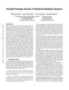
Domains. A domain is an infinitely countable set of values. All domains are enriched with a special value ∗ for representing NULL, the semantics of which refers to our lack of knowledge. Attributes and Relations. As usual, we assume a countable collection of attribute names. Each attribute Ai is characterized by a name and a domain dom(Ai ). A relation schema is a finite set of attributes and a relation instance is a finite subset of the Cartesian product of the domains of the relation schema. Context Parameters. Context is modeled through a finite set of special-purpose attributes, called context parameters (ci ). For a given application X, we can define its context environment CX as a set of n context parameters {c1 , c2 , . . . , cn }. Context State. In general, a context state is an assignment of values to context parameters. The context state at time instant t is a tuple with the values of the context parameters at time instant t, CSX (t) = {c1 (t), c2 (t), . . . cn (t)}, where ci (t) is the value of the context parameter ci at timepoint t. For instance, assuming location and weather as context parameters, a context state can be: CS(current) = {Acropolis, sunshine}. Hierarchies for Attributes. It is possible for an attribute to participate in an associated hierarchy of levels of aggregated data i.e., it can be viewed from different levels of detail. Formally, an attribute hierarchy is a lattice of attributes – called levels for the purpose of the hierarchy – L = (L1 , . . . , Ln , ALL). We require that the upper bound of the lattice is always the level all, so that we can group all the values into the single value � all� . The lower bound of the lattice is called the detailed level of the parameter. For instance, let us consider the hierarchy location of Fig. 2. Levels of location are Region, City, Country, and all. Region is the most detailed level. Level all is the most coarse level for all the levels of a hierarchy. Aggregating to the level all of a hierarchy ignores the respective parameter in the grouping (i.e., practically groups the data with respect to all the other parameters, except for this particular one).
All Country
City
Region
All Greece
Athens Acropolis
Salonica Kefalari
Polichni
Fig. 2. Hierarchies on location.
The relationship between the values of the context levels is achieved through L2 2 the use of the set of ancL L1 functions. A function ancL1 assigns a value of the domain of L2 to a value of the domain of L1 . For instance, ancCity Region (Acropolis) = Athens. A formal definition of these hierarchies can be found in [2].
Dynamic and Static Context Parameters. We discriminate between two kinds of context parameters: (a) static and (b) dynamic context parameters. Static context parameters take as value a simple value out of their domain. Dynamic context parameters on the other hand, are instantiated by the application of a function, the result of which is an instance of the domain of the context parameter. In our example, we assume that weather is a static parameter, i.e., each new value for weather derives from an explicit update. On the other hand, location� s values depends on time. The location is a function of time and in that way, we can compute the value of this parameter at the point we want to use it, without the need for continuous updates. 3.2
Contextual Preferences
In this section, we define how a context state affects the results of a query. In our model, each user expresses his/her preference by providing a numeric score between 0 and 1 [3]. This score expresses a degree of interest, which is a real number. Value 1 indicates extreme interest. In reverse, value 0 indicates no interest for a preference. The special value � for a preference, means that there is a user’s veto for the preference. Furthermore, the value ∗ represents that any value is acceptable. More specifically, we divide preferences into basic (concerning a single context parameter) and aggregate (concerning a combination of context parameters): – Basic preferences. Each basic preference is described by (a) a context parameter ci , (b) a set of non-context parameters Ai , and (c) a degree of interest, i.e., a real number between 0 and 1. So, for the context parameter ci , we have: pref erencebasici (ci , Ak+1 , . . . , An ) = interest scorei – Aggregate preferences. Each aggregate preference is derived from a combination of basic preferences. The aggregate preference is expressed by a set of context parameters ci and a set of non-context parameters Ai , and has a degree of interest (pref erence(c1 , . . . ck , Ak+1 , . . . , An ) = interest score). The interest score of the aggregate preference is a value function of the individuals scores (the degrees of the basic preferences). The value function prescribes how to combine basic preferences to produce the aggregate score, according to the user’s profile. Users define in their profile how the basic scores contribute to the aggregate, giving a weight to each context parameter. So, if the weight for a context parameter is wi the interest score will be: interest score = w1 ∗ interest score1 + . . . + wk ∗ interest scorek . In our motivating example, there are two context parameters, location and weather. Also, the set of non-context parameters are attributes about restaurants and users (in this case the user is M ary), that are stored in the database. From M ary � s profile we know that when she is at Acropolis she gives at the restaurant BeauBrummel the score 0.8, and when the weather is cloudy the same restaurant has score 0.9. In order to explain M ary � s high scores to the above preferences, we refer that the restaurant BeauBrummel is located in Athens,
near Acropolis, and M ary likes to eat f rench cuisine when the weather is cloudy (BeauBrummel has f rench cuisine). So, the basic preferences are: pref erencebasic1 (Acropolis, BeauBrummel, M ary) = 0.8 and pref erencebasic2 (cloudy, BeauBrummel, M ary) = 0.9 In this way, if the weight of location is 0.6 and the weight of weather is 0.4, the preference has score: 0.6 ∗ 0.8 + 0.4 ∗ 0.9 = 0.84 (from the above value function). Thus, we have: pref erence(Acropolis, cloudy, BeauBrummel, M ary) = 0.84.
4
The Storage Model
There is a straightforward way to store our context and preference information in the database. We organize preferences as data cubes, following the OLAP paradigm [2]. We discuss the implementation of our context model in relational DBMS structures. First, we discuss the storage of preferences and then the storage of attribute hierarchies. Location
User
Weather
User
Restaurants
Restaurants
Fig. 3. Data cubes for each context parameter.
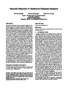
Storing Basic Preferences. In our model, we store basic user preferences in hypercubes, or simply, cubes. The number of data cubes is equal with the number of context parameters, i.e., we have one cube for each parameter, as shown in Fig. 3. In each cube, there is a dimension for restaurants, a dimension for users and a dimension for the context parameter. In each cell of the cube, we store the degree of interest for a specific preference. So, we can have the knowledge of score for a user, a restaurant and a context parameter. Formally, a cube is defined as a finite set of attributes C = (AC , A1 , . . . , An , M ), where AC is a context parameter, A1 , . . . , An are non-context attributes and M is the interest score. The values of a cube are the values of the corresponding preference rules. A relational table implements such a cube in a straightforward fashion. The primary key of the table is AC , A1 , . . . , An . If dimension tables representing hierarchies exist (see next), we employ foreign keys for the attributes corresponding to these dimensions. Our schema which is a modification of the classical star schema is depicted in Fig. 4. As we can see, there are two fact tables, F act Location and F act W eather. The dimension tables are: U sers and Restaurants. These are dimension tables for both fact tables.
Fact_Weather Restaurants rid
rid
uid
name
Users
weather
uid
score
phone region cuisine
name phone address
Location
e−mail
lid
Fact_Location
country
rid
city
uid
region
lid score
Fig. 4. The two fact tables of our schema (one for each context parameter) and the dimension tables for U sers and Restaurants.
Storing Context Hierarchies. An advantage of using cubes to store user preferences is that they provide the capability of using hierarchies to introduce different levels of abstractions of the captured context data [4]. In that way, we can have a hierarchy on a given context dimension. Context dimension hierarchies give to the application the opportunity to use a combination of data between the fact and the dimension tables on one of the context parameters. The typical way to store data in databases is shown in Fig. 5 (left). In this modeling, we assign an attribute for each level in the hierarchy. We also assign an artificial key to efficiently implement references to the dimension table. The contents of 2 the table are the values of the ancL L1 functions of the hierarchy. The denormalized tables of this kind, participating in a database schema often called a star schema suffer from the fact that there exists exactly one row for each value of the lowest level of the hierarchy. Therefore, if we want to express preferences at a higher level of the hierarchy, we need to extend this modeling (assume for example that we wish to express the preferences of M ary when she is in Cyprus, independently of the specific region, or city of Cyprus she is found at). To this end, in our model, we use an extension of this approach, as shown in the right of Fig. 5. In this kind of dimension tables, we introduce an extra tuple for each value at any level of the hierarchy. We populate attributes of lower levels with N U LLs. To explain the particular level that a value participates at, we also introduce a level indicator attribute. Dimension levels are assigned attribute numbers through a topological sort of the lattice.
Country
Level
G_ID
Region
City
1
Acropolis
Athens
Greece
1
2
Kefalari
Athens
Greece
1
3
Polichni
Salonica
Greece
1
... G_ID
Region
City
1
Acropolis
Athens
Greece
2
Kefalari
Athens
Greece
3
Polichni
Salonica
Greece
...
Country
101
NULL
Athens
Greece
2
102
NULL
Salonica
Greece
2
120
NULL
NULL
Greece
3
121
NULL
NULL
Cyprus
3
... ...
Fig. 5. A typical (left) and an extended dimension table (right).
Storing the Value Functions. The computation of aggregate preferences refers to the composition of simple basic preferences, in order to compute the aggregate one. The technique used for this involves using weights for each of the parameters. Each aggregate preference involves (a) a set of k context parameters -i.e., cubes and (b) a set of n non-context parameters, common to all context cubes: pref erence(c1 , . . . ck , Ak+1 , . . . , An ) = interest score The non-context parameters pin the values of the aggregate scores to specific numbers and then, the individual scores for each context parameter are collected from each context table. Recall that the formula for computing an aggregate preference is: interest score = w1 ∗ interest score1 + . . . + wk ∗ interest scorek . Therefore, the only extra information that needs to be stored concerns the weights employed for the computation of the formula. To this end, we employ a special purpose table AggScores(wC1 , . . . , wCk , Ak+1 , . . . , An ). The value for each context parameter wCi is the weight for the respective interest score and the value for each non-context attribute Aj is the specific value uniquely determining the aggregate preference. For instance, in our running example, the table AggScores has the attributes Location weight, W eather weight, U ser and Restaurant. A record in this table can be (0.6, 0.4, Mary, Beau Brummel). Assume that from M ary � s profile, we know that Beau Brummel has interest score at the current location 0.8 and at the current weather 0.9, then, the aggregate score is: 0.6 ∗ 0.8 + 0.4 ∗ 0.9 = 0.84
5
Querying Context
In this section, we classify the query operations that can be posed to our contextaware DBMS, by exploiting the combined information on preferences and context. Querying Simple Preferences. Firstly, there are queries executed without a need for the computation of the aggregate score. In this category of queries, users explicitly define that they are not interested in specific context parameters. For example, the following query computes the users’ preferences directly. Query 1 Look for M ary � s most preferable restaurants in Athens, independently of the status of weather. In SQL, the query is: – SELECT R.name, F L.score FROM Users U, Restaurants R, F act Location FL, Location L WHERE U.uid = F L.uid AND R.rid = F L.rid AND L.lid = F L.lid AND U.name =� M ary � AND L.region =� Athens� ORDER BY FL.score DESC; Another similar query would be “Look for the users in Athens that prefer restaurant Beau Brummel independently of weather” that can be used for example to advertise a specific restaurant in the context of “Athens”. Querying with Aggregate Scores. Another useful operation is the computation of aggregate scores from simple ones. For example, the following query needs to compute the aggregate score: Query 2 Look for M ary � s most preferable restaurants (in the current context).
The execution of Query 2 leads to the execution of the following subqueries (we suppose that CS(current) = {Acropolis, sunshine}): – SELECT R.name, F L.score FROM Users U, Restaurants R, F act Location FL, Location L WHERE U.name =� M ary � AND U.uid = F L.uid AND R.rid = F L.rid AND L.lid = F L.lid AND current location =� Acropolis� ; and – SELECT R.name, F W.score FROM Users U, Restaurants R, F act W eather FW WHERE U.name =� M ary � AND U.uid = F W.uid AND R.rid = F W.rid AND current weather =� sunshine� ; Using the results of subqueries, we calculate the aggregate scores for restaurants using the value function, as described above. In this case, we have the most preferable Mary’s restaurants in decreasing order. Traditional OLAP operators. OLAP provides a principled way of querying information. The traditional techniques for relational querying are enriched with special purpose query operators, such as roll-up and drill-down [5, 2]. – Slice-n-Dice. The dice operator on a data set corresponds to a selection (in the relational sense) of values on each dimension. A slice is a selection on one of the N dimensions of the cube. A dice operator can be implemented as a sequence of slices. Simple preference queries can be computed using slice operators. For instance, Query 1 can be implemented using slice operations on U ser and Location. – Roll-up. The roll-up operation provides an aggregation on one dimension. Here for example, a roll-up on location can generate a cube that uses cities instead of regions. – Drill-down. Similarly, drill-down is the reverse operation, i.e. when we have the result of a query which includes restaurants that are located in Athens, we can take a result that includes restaurants located at Acropolis, using the drill-down operator. Computing Aggregate Scores. The technique used for processing queries involving aggregate scores (e.g., Query 2 above) is the following. 1. First, a dice operator is executed on the context cubes. We select specific values for U sers and for the context parameter. For instance, for the first cube a selection could be on a value of location, e.g., Acropolis and for a value of user, e.g., M ary. 2. Second, having pinned all dimension attributes to a specific value, we have all the preference interest scores available. In fact, the individual scores for each context parameter are collected from each context table (although this practically involves a relational join on all non-context parameters, it is quite more easy to simply collect the values from the respective cubes from a set of point queries over them). So, we can compute the aggregate score of a preference by using a value function (as described in the previous sections).
3. In the context of an OLAP session, the aggregate scores just computed for a user can be stored in a new transient cube. As with cubes concerning basic preferences, a cube concerning aggregate preferences has one attribute for each context and non-context parameter and an extra attribute for the interest score. Then, the user can reuse the result of a query, by just using the last cube, without executing all the above steps.
6
Related Work
Although, there is much research on location-aware query processing in the area of spatio-temporal databases, integrating other forms of context in query processing is a new issue. Context and Queries. In the context-aware querying processing framework of [6], there is no notion of preferences, instead context attributes are treated as normal attributes of relations. Query processing is divided into three-phases: query pre-processing, query execution and query post-processing. During query pre-processing, a query is further constrained by adding constraints that may include context attributes and any contextual attributes are bound to exact values. After query execution, at the query post-processing phase, the results may be sorted by observing predefined rules. This framework is orthogonal to our approach and a potential extension of our work includes enriching our model with constraints involving context attributes. Storing context data using data cubes, called context cubes, is proposed in [4] for developing context-aware applications that use archive sensor data. In this work, data cubes are used to store historical context data and to extract interesting knowledge (such as rules, regularities, constraints, patterns) from large collections of context data. In our work, we use data cubes for storing context-dependent preferences and answering related queries. Finally, context has been used in the area of multidatabase systems to resolve semantic differences, e.g., [7–9] and as a general mechanism for partitioning information bases [10]. Preferences in Databases. In this paper, we use context to confine database querying by selecting as results the best matching tuples based on the user preferences. The research literature on preferences is extensive. In particular, in the context of database queries, there are two different approaches for expressing preferences: a quantitative and a qualitative one. With the quantitative approach, preferences are expressed indirectly by using scoring functions that associate a numeric score with every tuple of the query answer. In our work, we have adapted the general quantitative framework of [3], since it is more easy for users to employ. In the quantitative framework of [11], user preferences are stored as degrees of interest in atomic query elements (such as individual selection or join conditions) instead of interests in specific attribute values. Our approach can be generalized for this framework as well, either by including contextual parameters in the atomic query elements or by making the degree of interest for each atomic query element depend on context. In the qualitative approach (for example, [12]), the preferences between the tuples in the answer to a query are specified directly, typically using binary preference relations. For example,
one may express that restaurant1 is preferred from restaurant2 if their opening hours are the same and its price is lower. This framework can also be readily extended to include context. For instance, one may express that restaurant1 is preferred from restaurant2 if their opening hours are the same, its price is lower and it is closer to the current user’s location.
7
Summary
The use of context is important in many applications such as in pervasive computing where it is important that users receive only relevant information. In this paper, we consider integrating context with query processing, so that when a user poses a query in a database, the result depends on context. In particular, each user indicates preferences on specific attributes of a relation. Such preferences depend on context. We store preferences in data cubes and show how OLAP techniques can be used to compute context-aware queries, that is queries whose results depend on context.
References 1. Dey, A.K.: Understanding and Using Context. Personal and Ubiquitous Computing 5 (2001) 2. Vassiliadis, P., Skiadopoulos, S.: Modelling and Optimisation Issues for Multidimensional Databases. In: Proc. of 12th International on Advanced Information Systems Engineering,(CAiSE 2000), Stockholm, Sweden, June 5-9, 2000. Volume 1789 of Lecture Notes in Computer Science., Springer (2000) 482–497 3. Agrawal, R., Wimmers, E.L.: A Framework for Expressing and Combining Preferences. In: Proc. of SIGMOD. (2000) 4. Harvel, L., Liu, L., Abowd, G.D., Lim, Y.X., Scheibe, C., Chathamr, C.: Flexible and Effective Manipulation of Sensed Contex. In: Proc. of the 2nd Intl. Conf. on Pervasive Computing. (2004) 5. Gray, J., Chaudhuri, S., Bosworth, A., Layman, A., Reichart, D., Venkatrao, M., Pellow, F., Pirahesh, H.: Data Cube: A Relational Aggregation Operator Generalizing Group-By, Cross-Tab, and Sub-Totals. Data Mining and Knowledge Discovery 1 (1997) 6. Feng, L., Apers, P., Jonker, W.: Towards Context-Aware Data Management for Ambient Intelligence. In: Proc. of the 15th Intl. Conf. on Database and Expert Systems Applications (DEXA). (2004) 7. Kashyap, V., Sheth, A.: So Far (Schematically) yet So Near (Semantically). In: Proc. of IFIP WG 2.6 Database Semantics Conference on Interoperable Database Systems (DS-5). (1992) 8. Ouksel, A., Naiman, C.: Coordimnating Context Building in Heterogeneous Information Systems. J. Intell Inf Systems 3 (1993) 9. Sciore, E., Siegel, M., Rosenthal, A.: Using Semantic Values to Facilitate Interoperability Among Heterogeneous Information Systems. ACM TODS (1994) 10. Mylopoulos, J., Motschnig-Pitrik, R.: Partitioning Information Bases with Contexts. In: Proc. of CoopIS. (1995) 11. Koutrika, G., Ioannidis, Y.: Personalization of Queries in Database Systems. In: Proc. of ICDE. (2004) 12. Chomicki, J.: Preference Formulas in Relational Queries. TODS 28 (2003)