vr = v# = 0; v' = iri sin# at ICB; vr = v# = v' = 0 at CMB: (6). The angular velocity of the inner core rotation i can be obtained from the impuls momentum equation.
ON THE APPLICATION OF GRID-SPECTRAL METHOD TO THE SOLUTION OF GEODYNAMO EQUATIONS P. HEJDA AND I. CUPAL
Geophysical Institute, Acad. Sci, 141 31 Prague, Czech Republic AND M. RESHETNYAK
Institute of the Physics of the Earth, Russian Acad. Sci, 123810 Moscow, Russia
1. Introduction The geodynamo process of magnetic eld generation occurs in the outer core of the Earth and is described by 3D MHD-equations. The focus of this paper is on a numerical solution and thus the equations will be considered, without the loss of generality, in a simple Boussinesq approximation. Denoting B the magnetic eld, v the velocity, p the pressure and T the temperature, the dimensionless equations read
@ B = r� (v � B) + r2 B; @t
(1)
Ro( @@tv + v �rv) = rp + F + E r2v;
(2)
@T + v �r(T + T ) = q r2 T; o @t r� B = 0; r� v = 0;
where F is the sum of Archimedean, Corioliss and Lorenz forces
F = qRaTr1r (v � 1z ) + �(r� B) � B;
(3) (4) (5)
2
P. HEJDA ET AL.
and where the following dimensionless numbers are introduced
� [Ekman number]; E = 2 L 2 2
B0 [The Elsasser number]; � = 2 ���
Ro = 2 �L2 [Rossby number]; q = ��
o �L [Rayleigh number]: Ra = �g2 �
[Roberts number];
Here � = (�� ) 1 is the magnetic di�usivity, � the permeability, � the electrical conductivity, � the mean density, � the kinematic viscosity, is the Earth's rotation rate, � is the coe�cient of volume expansion, � is the unit of temperature and � represents the eddy thermal di�usivity. The Earth's core radius is the unit of length, L, the velocity is measured by �=L, the unit of time is L2=� and B0 is the mean magnetic eld within the Earth's outer core. The most frequently used method of solution was outlined in the 1950's by Bullard and Gellman (1954). It consists of decomposition of vector elds into toroidal and poloidal parts spectral transformation with spherical harmonics in angular coordinates special functions (Chebyshe� polynomials, Bessel functions) or nite di�erences in radial direction. In spite of the general decrease of popularity of spectral methods in the 1970's in favour of nite di�erences or nite elements, the above method has kept its privileged position in the planetary magnetohydrodynamics because of its indisputable advantages: the condition of non-divergence is automatically satis ed 'boundary conditions' on the axis of rotation are involved in the properties of spherical harmonic functions magnetic eld can be easily tted to an outer source-free potential eld. A di�erent approach was used only for some 2D models (Jepps, 1975; Braginsky, 1978; Braginsky and Roberts, 1987; Cupal and Hejda, 1989; Anufriev et al., 1995; Jault, 1995; Anufriev and Hejda, 1998) In this approach, the resolution into toroidal and poloidal parts is retained but the resulting equations are approximated by nite di�erences scheme on a 2D spherical grid in the meridional plane. In our new method for 3D hydromagnetic dynamo we build on our previous positive experience with nite di�erences approximation in the meridional plane. It is combined with the spectral method in �-component.
APPLICATION OF GRID-SPECTRAL METHOD
3
Similar method, except in cylindrical coordinates, was developed by Nakajima and Roberts (1995) for kinematic dynamo.
2. Grid-spectral approach Vector elds are represented in the form
0 Fsm 1 0 F 1 M 0 Fcm 1 r r r X F(r; �; '; t) = @ F� A = @ F�c m A cos m' + @ F�s m A sin m'; F'
m=0
and scalars functions analogously as
F (r; �; '; t) =
M X m=0
F'c m
F's m
F c m cos m' + F s m sin m':
Since spherical coordinates are used, not only boundary conditions on the physical boundaries must be formulated (the inner-outer core boundary, ICB, and the core-mantle boundary, CMB), but also conditions along the axis of rotation and (for magnetic eld) in the center of the sphere. Using the properties of analytical scalar or vector functions for � ! 0, � ! � we obtain @Frm = F m = F m = 0; for m = 0; � ' @� m @F m Frm = @F@�� = @�' = 0; for m = 1; Frm = F�m = F'm = 0; for m > 1:
The boundary conditions for scalar functions coincide with those for component r. The spherical components of the dipolar magnetic eld are not de ned in the center of the sphere. It would cause problems in the numerical solutions and thus the new variable b = rB is introduced. This variable is equal to zero for all spherical components at the center of the sphere. The toroidal-poloidal decomposition is not used in this method and the validity of eqs.(4) and (5) is not automatically satis ed. Their respective roles in the magnetic induction equation (1) and in the uid momentum equations (2) are di�erent. If the initial magnetic eld were non-divergent, the exact solution of (1) would preserve the same property. However, there is a danger that the non-divergence of the solution will deteriorate due to rounding errors during the numerical process. Therefore, eq. (1) is integrated only for components � and ' and the r-component is computed using the condition (4). The detailed description of the numerical solution of the magnetic induction equation, including numerical tests, can be found in Hejda and Reshetnyak, 1999 and 2000.
4
P. HEJDA ET AL.
3. Fractional step method With regards to the uid momentum equation (2), the incompressibility condition (5) is a constraint in the space of possible solutions and it is related in the implicit form to the pressure eld. The solution must further satisfy the boundary conditions. We will consider non-slip boundary conditions with possible rotation of the solid inner core, i.e.
vr = v# = 0; v' = i ri sin # at ICB; vr = v# = v' = 0 at CMB:
(6)
The angular velocity of the inner core rotation i can be obtained from the impuls momentum equation
i Z� h @ � v' � @
i sin2 �d� + Br B' Ro = I @t = 2�ri3 Er @r r r = r r =r 0 i
(7)
i
where I = 158 �ri5 is the moment of inertia of the inner core. The equation (7) is reduced to the balance between viscous and magnetic torque when I is ignored. The velocity boundary conditions will be further denoted simply as v^ for clear explanation of the algorithm, which is a variation of the Fractional step method (Heinrich and Pepper,1999). The velocity is sought at each time step n in the form of a sum of two parts:
vn = Un + un ; where Un+1 is obtained in the rst substep as the solution of eq.(2) without pressure term n+1 n Ro U �t v = Ro vn �rvn + Fn + E r2vn with the boundary conditions U�n+1 = �t @pn =@� + v^� and Urn+1 = v^r = 0 at ICB and CMB. Here � denotes tangential components # or '.
In the second substep the correction of the velocity is computed using the pressure term. Applying r� to (2) the Poisson equation
r2pn+1 = r� ( Rovn �rvn + Fn + E r2vn) = (�t) 1r� Un+1 is obtained. It is solved with boundary condition @pn+1 =@r = 0 at ICB and CMB. The correction of the velocity is then
un+1 = �trpn+1 :
APPLICATION OF GRID-SPECTRAL METHOD
5
Figure 1. The snapshot of the solution of the dynamo equation with an eastward rotating inner core i = 36:4. The dashed contours relate to the negative values. It can be easily veri ed that vn+1 is incompressible and satis es (2) and (6).
4. Computer code and numerical tests The form of the equation of temperature conductivity (3) is similar to the components of the magnetic induction equation (1) and its solution does not represent any additional di�culties. The computer code was written in Fortran 77 and implemented on PC Pentium III. The power of the computer has allowed us to carry out the tests in the so-called 2.5D approximation, i.e. just for a few modes in '. As an example of the solution of the geodynamo model the equation are solved for m � 2 using the following parameters: � = 1; q = 1:82; Ro = 2 � 10 3 ; E = 2 � 10 3 ; Ra = 3 � 102: The temperature pro le within the outer core is T0 = ri1=r r 1 : i An interesting feature of the solution is that by solving the equation(7) with non-zero I we obtain an eastward rotation of the inner core i that
6
P. HEJDA ET AL.
uctuates (in time) around the value 20. However, when I = 0 is assumed in eq. (7) the inner core rotates westward and the value of i uctuates around the value -15. A snapshot of the time dependent solution with I 6= 0 is shown in the gure 1. Even though the inner core rotates eastward the azimuthal component of velocity at the core-mantle boundary is negative (westward drift), particularly at the equator and polar regions.
5. Conclusion Several codes for solution of hydromagnetic dynamos in a rotating spherical shell have been recently available, but all of them are based on a similar (spectral) approach. Therefore, it is useful to have an alternative method. This recent contribution is a follow-up to our studies devoted to the kinematic dynamo and presents the rst test solutions of the full set of hydromagnetic dynamo equations. The method is applicable to the solution of the geodynamo models. However, the question remains whether we will still be able to obtain the solution when choosing all parameters closer to the real parameters of the Earth's core, particularly the Ekman number, whose real values are assumed to be under E = 10 12 .
References
Anufriev, A.P., Cupal, I. and Hejda, P. (1995) The weak Taylor state in an �!-dynamo. Geophys. Astrophys. Fluid. Dyn., 79, 125{145. Anufriev, A.P. and Hejda, P. (1998) E�ect of the magnetic eld at the inner core boundary on the ow in the Earth's core. Phys. Earth Planet. Inter., 106, 19{30. Braginsky, S.I. (1978) Nearly axially symmetric model of the hydrodynamic dynamo of the Earth II. Geomag. Aeron., 18, 225{231. Braginsky, S.I. and Roberts, P.H. (1987) A model-Z geodynamo. Geophys. Astrophys. Fluid. Dyn., 38, 327{349. Bullard, E.C. and Gellman, H. (1954) Homogeneous dynamos and terrestrial magnetism. Phil. Trans. R. Soc. Lond., A 247, 213{278 Cupal, I. and Hejda, P. (1989) On the computation of a model-Z with electromagnetic core-mantle coupling. Geophys. Astrophys. Fluid. Dyn., 49, 161{172. Heinrich, C.J., Pepper, D.W. (1999) Intermediate nite element method, Taylor & Francis, New York, pp.1-585 Hejda, P., Reshetnyak, M. (1999) A grid-spectral method of the solution of the 3D kinematic geodynamo with the inner core. Studia geoph. et. geod., 43, 319{325 Hejda, P., Reshetnyak, M. (2000) The grid-spectral approach to 3-D geodynamo modelling. Computers & Geosciences, 26, 167{175 Jault, D. (1995) Model Z by computation and Taylor's condition. Geophys. Astrophys. Fluid. Dyn., 79, 99{124. Jepps., S.A. (1975) Numerical models of hydromagnetic dynamos. J. Fluid. Mech., 67, 625{646. Nakajima, T. and Roberts, P.H. (1995) An application of mapping method to asymmetric kinematic dynamos. Phys. Earth Planet. Inter., 91, 53{61.