On the Combination of Constraint Programming and Stochastic Search: The Sudoku Case Rhydian Lewis Prifysgol Caerdydd/Cardiff University, Cardiff Business School, Colum Drive, Cardiff, WALES.
[email protected]
Abstract. Sudoku is a notorious logic-based puzzle that is popular with puzzle enthusiasts the world over. From a computational perspective, Sudoku is also a problem that belongs to the set of NP-complete problems, implying that we cannot hope to find a polynomially bounded algorithm for solving the problem in general. Considering this feature, in this paper we demonstrate how a metaheuristic-based method for solving Sudoku puzzles (which was reported by the same author in an earlier paper), can actually be significantly improved if it is coupled with Constraint Programming techniques. Our results, which have been gained through a large amount of empirical work, suggest that this combination of techniques results in a hybrid algorithm that is significantly more powerful than either of its constituent parts
1
Introduction
Sudoku is a popular puzzle that appears regularly in a variety of newspapers, books, and puzzle magazines worldwide. Although originating in the United States in the late 1970s, it was actually in Japan in the 1980s that the puzzle gained mainstream popularity. It was also here where it was given the name “Sudoku”, which can be loosely translated in English as “solitary number”. In its simplest form, Sudoku can be defined as follows. Given an n2 × n2 grid divided into n2 distinct n × n boxes (denoted by the bold lines in fig. 1), the aim is to fill the grid so that three separate criteria are met: 1. Each row of cells contains the integers 1 through to n2 exactly once; 2. Each column of cells contains the integers 1 through to n2 exactly once; 3. Each n × n box contains the integers 1 through to n2 exactly once. In this paper we will refer to the value of n as the order of a puzzle. Typically some of the cells in a Sudoku grid will have been pre-filled by the puzzle master (see fig. 1). The player will then use these to logically determine the values for other cells in the grid, eventually allowing him-or-her to complete the puzzle. As can be imagined, how many and which cells the puzzle-master chooses
8 1 8 6 7 9 6
2 3 5 7 1 9 6 7 4 1 8 1 4 2 4 8 4 5 9 3
5 Fig. 1. Example of an order-3 Sudoku puzzle. This particular grid is logic-solvable.
to fill will therefore be particularly important if the puzzle is to be enjoyable for the player. Generally speaking, a “good” puzzle (from the player’s perspective) should be configured in such a way so that is logic-solvable – that is, the player should be able to complete the puzzle in a logical sequence of steps using forwardchaining logic only (obviously the deductive abilities of different players will vary). In particular, a player should not usually be required to make random choices, especially when the grid is still quite empty, because if this guess turns out to be wrong, he-or-she will then have to go through the unsatisfying process of backtracking and re-guessing. For these reasons “good” Sudoku puzzles tend to have just one possible solution in each case. From a computing perspective, the manual methods by which human players go about solving Sudoku puzzles (albeit unbeknown to most of them) closely follow simple Constraint Programming (CP) methods – each of the n4 cells in the grid represents an integer variable which, initially, will have a domain of 1 through to n2 . Constraints can then be added in the form of “alldifferent” constraints [1] (i.e. “all of the variables in row three should have different values”, etc.), and by using the pre-filled cells in the grid (e.g. “because 5 appears in row three, none of the unfilled cells in row three can contain a 5”, etc.). Combinations of such constraints will reduce the domain-sizes of some of the variables and, if an appropriate propagation scheme is used, the puzzle can then (hopefully) be completed. (See the work of Simonis [2] for an example application of advanced CP techniques to logic-solvable puzzles of order-3.) It is worth noting, however, that not all puzzles will have the logic-solvable property. Indeed, Sudoku has been proved to belong to the class of NP-complete problems [3], implying that we cannot hope to find a polynomially bounded algorithm for solving all problem instances (unless, of course, P = NP). In other words, we can be fairly sure that there will be many problem instances where the exclusive use of logical rules will not be enough and some sort of search will also be required. For this reason, many existing automatic Sudoku solvers also include
branch-and-bound search mechanisms, such as the Sudoku Solver by Logic.1 However, for this sort of approach to be successful there will, of course, also be a reliance on the search space being a manageable size. Indeed, in situations where this is not so – perhaps because the grid is still quite empty and/or because the puzzle is of a high order – then the potential timing implications of such searches might turn out to be impractical. Given the above, in a previous paper [4] we suggested that it might also be useful to consider other types of search methods with Sudoku. Consequently, we proposed a stochastic approach based around Simulated Annealing (SA). In the next section we will describe this algorithm and its general characteristics (as reported in [4]). Subsequently, we will then suggest a way in which this algorithm might be coupled with a simple CP procedure to form a more powerful hybrid algorithm. In Section 3 we will then carry out a number of experiments to compare our original SA algorithm with this new approach and will discuss our results. Finally, Section 4 will conclude the paper.
2
A Hybrid Algorithm for Solving Sudoku
In the following descriptions, a grid cell will be described as fixed when its value is definitely known, either because it has been defined in the problem instance or, in the case of our hybrid algorithm, because its value has been determined by our CP procedure (to be described in Section 3). Cells whose values are undetermined will be described as unfixed. The SA algorithm operates as follows. Given a problem instance of order n, the algorithm first creates an initial solution by assigning a value to each of the unfixed cells in the grid. This is done randomly, but in such a way so that each box ends up containing the values 1 through to n2 exactly once. Creating an initial solution in this way guarantees that the third criteria of Sudoku is met; however, it also means that the grid may well feature violations of the remaining two criteria. A suitable cost function is thus: 2
n X i=1
2
r(i) +
n X
c(j)
(1)
j=1
where r(i) and c(j) represent the number of values, 1 through to n2 , that are not present in the ith row of cells and the jth column of cells respectively. An optimal (i.e. valid) solution will thus have a cost of zero. In order to try and find an optimal solution, a neighbourhood operator is then used that randomly selects two unfixed cells in the same box, and swaps their contents. Following standard SA methods, a swap is then accepted (a) if it causes the cost to drop, or (b) with a probability exp(−δ/t), where δ represents the proposed change in cost and t is the current temperature of the system. During a run t is slowly reduced from an initial value t0 according to a geometric 1
Available at http://www.sudokusolver.co.uk/index.html
cooling schedule. A simple reheating function is also used that resets t to t0 when the algorithm considers itself to be caught in a local minimum. Note that the neighbourhood operator ensures that the third criterion of Sudoku is always met. This means that that the total size of the search space is: n Y n Y
f (i, j)!
(2)
i=1 j=1
where f (i, j) indicates the number of unfixed cells in the box in the ith row of boxes and jth column of boxes. In [4], this SA algorithm was applied to a large number of solvable problem instances using a generator that was able to closely control the proportion of fixed cells in a grid (this will also be used in Section 3). Results indicated that, similarly to many other combinatorial optimisation problems (e.g. [5, 6]), Sudoku also features an “easy-hard-easy” phase transition with solvable instances. In other words, the SA algorithm is generally able to discover an optimal solution when presented with instances containing very low or very high proportions of fixed cells, but at the boundary of these two extremes there occur instances that the algorithm finds more difficult to solve. The suggested reasons for this phase transition are as follows: When the proportion of fixed cells in a grid is low, then according to eq. (2) there will be a large search space for the algorithm to navigate. However, there will also be a very large number of optimal solutions within this search space.2 Consequently, the algorithm will nearly always be able to find one of these in a reasonable amount of time. For grids with high proportions of fixed cells, meanwhile, although there will only be a very small number of optimal solutions (and perhaps only one), the search space will be much smaller. Additionally, it is also likely that solutions to these highly constrained instances will tend to lie at the bottom of deep local minima (with a strong basin of attraction), thus also allowing easy discovery by the algorithm. However, instances at the boundary of these two extremes cause the algorithm more problems. First, the search spaces for these instances will still be relatively large, but they will also tend to admit only a small number of solutions. Second, because of their moderate numbers of constraints, the fitness landscapes will also tend to feature more plateaus and local minima, making things even more difficult for the algorithm. (See also the work of Cheeseman et al. [8]) From these explanations it is easy to see that, from the point-of-view of a stochastic search approach, an important contributing factor for an instance being “hard” is a large search space. However, it is fairly obvious that one way that we might go about alleviating this factor is by first determining the contents of as many cells as possible before applying such an algorithm. This is the approach that our new hybrid algorithm will take here. Given a particular problem instance, a simple CP procedure will first be applied which will fill-in 2
It has been calculated by Felgenhauer and Jarvis [7], for example, that there are 6,670,903,752,021,072,936,960 different optimal solutions for order-3 grids.
and fix as many cells as possible. Then, once this stage has been completed the resultant partial solution will then be passed over to our original SA algorithm, which will operate in the manner that we have described.
3
Experimental Analysis
In order to compare the performance of the two algorithms, experiments were carried out on a large number of solvable problem instances of various orders. In Section 3.1 we will describe the experiments that we conducted on randomlyformed problem instances (i.e. ones that are not necessarily logic-solvable). In Section 3.2 we will then present results that were gained when using collections of publicly available puzzles. In all experiments the CP procedure that was used in conjunction with our hybrid algorithm operated by following the 5 steps given below. This procedure is deterministic. 1. For each unfixed cell in the grid, construct a list of possible values that this cell could contain by examining the contents of the cell’s row, column, and box; 2. If any of these lists contains just one value, then insert this value into the cell, mark it as fixed, and go back to step 1; 3. Look at each row in turn. If any cell’s list in a particular row contains a value x that does not occur in any of the other cells’ lists on the same row, then insert x into this cell, mark the cell as fixed, and go back to step 1; 4. Repeat step 3 for each column and also each box; 5. If we are here, then the procedure cannot fix any further cells, and so end. 3.1
Solving Random Sudoku Grids
For our first set of experiments we used the same method of instance generation as in [4], which operates as follows: To start with, a full and optimal Sudoku grid of a given order is taken. Such a grid can be obtained from a variety of places such as the solution pages of a Sudoku book or newspaper, by calculating the puzzles “Root Solution” (see [4]), or by simply running the SA algorithm using a blank grid as a problem instance. In the next step of the procedure, this grid is then randomly shuffled using the following five operators: – – – – –
Transpose the grid (2 possibilities); Permute columns of boxes within the grid (n! possibilities); Permute rows of boxes within the grid (n! possibilities); Permute columns of cells within a column of boxes (n!n possibilities); and Permute rows of cells within a column of boxes (n!n possibilities).
Note that all of these shuffle operators preserve the optimality of the grid. Finally, a number of cells in the grid are then made blank by going through each cell in turn and deleting its contents with a probability 1 − p, where p is a parameter to be defined by the user. Obviously, this means that instances generated with a low p-value will have a low proportion of fixed cells (i.e. a fairly unconstrained problem instance), whilst larger values for p will give more constrained, full problem instances.
prop. of fixed cells after CP procedure
Before comparing the SA and hybrid algorithms, it is first worth taking a look at how our CP procedure is able to cope with the randomly generated instances unaided. This is shown in fig. 2. Here, we can witness the clear pattern between the proportion of fixed cells in the initial problem instance, and the proportion of cells that are fixed after the CP procedure has been applied. As is shown, for very low p-values (0 to approximately 0.2) the CP procedure is not able to do anything at all, because the near-blank grids that occur here do not provide enough clues for any further cells to be filled. Meanwhile, for pvalues of approximately 0.75 and above, because of the high proportion of fixed cells in the instances, the CP procedure is nearly always able to complete the puzzles. Finally, in-between these values, although the procedure is often unable to complete the puzzles, it is, however, usually able to fill some of the cells. Note that this procedure is also very quick to run – none of these trials took more than 0.03 CPU seconds (using Windows XP, with an Intel 3.2GHz processor and 1.99Gb of RAM).
1 0.8 0.6 0.4 no CP order-3 order-4 order-5
0.2 0 0
0.2 0.4 0.6 0.8 prop. of fixed cells in problem instance (p)
1
Fig. 2. The relationship between p and the proportion of fixed cells after an application of the CP procedure for problems of order 3, 4, and 5. Each individual point in the figure is a mean, calculated after runs on twenty problem instances of a specific p-value. The smooth lines were produced using Gnuplot’s sbezier function
In order to compare the SA and hybrid algorithms directly, we used same instance generator to perform the following experiments. For p-values of 0 to 1.0 (incrementing in steps of 0.05), twenty separate problem instances were first created. With each of these instances, twenty separate trials with both algorithms were then performed. This was done for instances of order-3 (91 cells), order-4 (256 cells), and order-5 (625 cells), using time limits of 2, 40, and 450 CPU seconds respectively. Finally, the SA in both algorithms was executed under the following conditions: – An intial temperature t0 was calculated by applying a small number of neighbourhood moves to the initial solution (in our case we used 100 moves). t0 was then set to the variance of the cost across these moves (see [9] for the theoretical foundations of this). P n Pn – At each temperature a total of ( i=1 j=1 f (i, j))2 neighbourhood moves were attempted, where f has the same interpretation as eq. 2. – The temperature was updated using a simple geometric scheme whereby ti+1 = αti . In our case, we set α = 0.99. – Finally, if no improvements in the cost were found for twenty successive temperatures, then the current temperature was reset to t0 , whereupon the algorithm would continue as before. Figure 3 shows the results of these experiments and displays, for each algorithm, their success rates and solution times for all of the tested p-values. The success rate indicates the proportion of runs where the algorithms were able to find an optimal solution within the specified time limits. The solution time indicates the average number of CPU seconds that it took to find a solution. (In cases where the success rate was less than 1.0, those runs where optimality was not found were not considered in the latter’s calculation.) Looking at the order-3 results first, we can see that both algorithms feature a 100% success rate across all of the instances and that, in both cases, lower values for p will generally require longer solution times (due to the noted fact that these instances will feature a larger search space). We can also see that for p-values of 0 through to 0.2, both algorithms feature roughly the same solution times. This is because, as we saw in fig. 2, with these instances the CP procedure will not usually be given sufficient clues in order to be able to fill any of the cells, and so the two algorithms are equivalent. For p-values of 0.25 up to around 0.7, however, we can see that the hybrid algorithm clearly shows shorter solution times, due to the fact that the CP procedure is able to fill some of the cells, therefore reducing the size of the search space for the SA algorithm. Moving our attention onto the results of the order-4 and order-5 experiments, similar patterns also emerge with the solution times. In the centre of both graphs we also witness dips in the success rates, indicating the presence of the phase transition region that we have mentioned in Section 2. As we noted in [4], it can also be seen that as puzzle order is increased, then the effects of the phase transition also become more pronounced. Note, however, that throughout the
phase transition the hybrid algorithm shows both higher success rates and also shorter solution times than the SA algorithm. According to a signed ranked test
1 1.4
Solution Time (SA) Success Rate (SA) Solution Time (Hybrid) Success Rate (Hybrid)
0.8
1 0.6 0.8 0.6
0.4
success rate
solution time (CPU seconds)
1.2
0.4 0.2 0.2 0
0 0
0.2
0.4 0.6 proportion of fixed cells (p)
0.8
1
30
1 Solution Time (SA) Success Rate (SA) Solution Time (Hybrid) Success Rate (Hybrid)
0.8
0.6 15 0.4 10 0.2
5
0
0 0
0.2
0.4 0.6 proportion of fixed cells (p)
0.8
1
250
1 Solution Time (SA) Success Rate (SA) Solution Time (Hybrid) Success Rate (Hybrid)
200 solution time (CPU seconds)
success rate
20
0.8
150
0.6
100
0.4
50
0.2
0
success rate
solution time (CPU seconds)
25
0 0
0.2
0.4 0.6 proportion of fixed cells (p)
0.8
1
Fig. 3. Comparison of the SA and hybrid algorithms’ performance with puzzles of order-3 (top), order-4 (middle), and order-5 (bottom).
the increases in the success rates across the various p-values were seen to be significant (with ≥ 95% confidence). 3.2
Solving Published Sudoku Grids
For our second set of experiments we also tested the SA and hybrid algorithms on a number of published instances that are known to have unique solutions. Our first set of order-3 puzzles was taken from the on-line resource provided by the Los Angeles Times [10]. These were published in the newspaper between January and March 2006 and all are known to be logic solvable. A second set of order-3 puzzles was also taken from [11]. This resource features a very large collection of different puzzles that each contain just 17 fixed cells, which is currently the known minimum for guaranteeing that an order-3 puzzle features exactly one solution. Finally, for completeness we also used the instance generator available at [12] to produce a number of order-4 and order-5 puzzles. In general, puzzles of this size are much less popular than order-3 puzzles and so our choices here were limited. For this reason, we advise the reader to show slight caution when interpreting these latter results, as this generator has not been scientifically verified. Table 1 contains the results of these experiments and displays the source of the puzzles, their order, the number of instances used each case (Inst.), the average proportion of fixed cells in the instances (Fixed), and the puzzles’ “grades”.3 For each algorithm we then present the corresponding success rates and solution times (with standard deviation), calculated in the same manner as in Section 3.1. For the hybrid algorithm, we also present the average proportion of fixed cells that occurred after the CP procedure was applied (Fixed0 ). All entries are an average of ten runs on each of the available instances – i.e. 10 × Inst. runs in each case. The same CPU time limits as Section 3.1 were also used. As can be seen, in all cases the hybrid algorithm features an equal or higher success rate than the SA algorithm. Additionally, in all but two of the instance sets, we can see that the hybrid algorithm also gives shorter solution times (the remaining two cases are due to sampling errors caused by the very low success rates). One interesting point to note from this table is the relatively low success rates when tackling the order-3 instances of [11]. In reality these instances might be the most difficult sorts of problem for a stochastic search approach, because they feature close to the largest possible search spaces for order-3 grids whilst also ensuring that only one possible solution exists. For similar reasons, we can also see that the success rates for both algorithms also drop as the order of the puzzles is increased (with the one anomaly being the order-4 “superhard” instances, which could be due to some feature of the problem generator). 3
Note that puzzle grades are probably superfluous here, because they tend to relate to the complexity of the logical techniques that a player needs to use in order to complete it. Additionally, the boundaries and adjectives that are used to define the different grades also vary from place to place.
Table 1. Performance Comparison of the SA and Hybrid Algorithms with Instances with Unique Solutions Instance Description Source Order Inst. Fixed
[10] [10] [10] [11] [12] [12] [12] [12] [12]
4
SA Performance Grade Suc. Rate
3 10 0.34 gentle 3 10 0.36 tough 3 10 0.34 diabolical 3 1000 0.21 n/a 4 10 0.40 easy 4 10 0.40 hard 4 10 0.49 superhard 5 10 0.46 easy 5 10 0.45 hard
0.99 0.95 0.82 0.01 0.04 0.10 0.91 0.01 0.00
Hybrid Performance
Sol. Time Fixed0 Suc. Rate
0.67 ± 0.1 0.76 ± 0.3 0.80 ± 0.3 1.41 ± 0.2 14.3 ± 7.5 20.3 ± 9.4 8.64 ± 6.6 165.9 ± 0.0 n/a
0.94 0.59 0.48 0.30 0.47 0.48 0.74 0.51 0.49
Sol. Time
1.00 0.05 ± 0.1 1.00 0.22 ± 0.2 0.99 0.49 ± 0.2 0.16 0.64 ± 0.5 0.24 25.8 ± 10.3 0.28 16.4 ± 8.6 1.00 2.18 ± 2.5 0.04 234.1 ± 23.2 0.00 n/a
Conclusions and Discussion
In this paper we have seen that our hybrid algorithm, which incorporates constraint programming and stochastic search, clearly outperforms the same stochastic search algorithm when used on its own. We have seen that the two techniques that make up this hybrid algorithm actually seem to complement one another, because it is evident that on the one hand, CP techniques have the potential to drastically improve the performance of the stochastic search algorithm, whilst on the other hand, the stochastic search algorithm can also be used to help CP-based approaches to solve a much wider range of instances (i.e. those that are not necessarily “logic-solvable”). Indeed, it is also likely that if we were to improve either aspect of the hybrid algorithm (e.g., by using more advanced deduction techniques such as the “swordfish” and “X-wing” rules [13], or by using more sophisticated search techniques), then the overall performance of the hybrid algorithm would also subsequently improve. One interesting aspect of this work is the observation that our CP procedure allows the possibility of moving a problem instance away from the phase transition region, thus making it easier for the SA algorithm to solve. However, if this is the case, then we might ask whether it is also possible for the same procedure to move some instances into the phase transition region, making them harder to solve. We believe the answer to this question to be negative. This is because, as we have seen, the CP procedure will only ever fix a cell if it has deduced its contents with absolute certainty. Thus, although the procedure might be able to reduce the search space size by adding additional constraints, it will not reduce the number of solutions within this space, and its actions may well lead to a reduction in the number and/or size of plateaus in the fitness landscape. It is likely, therefore, that the instance will become easier to solve in general. Considering future work, it is interesting to note that Sudoku can also be modelled as a graph colouring problem. This is done by considering each of the n4 cells in a grid as a node, and then adding edges between any two nodes
corresponding to a pair of cells in the same row, column, and/or box (meaning that the n2 nodes occurring in each row/column/box will form a clique of size n2 .) Further edges can then also be added due to the pre-filled cells that are supplied with the puzzle – for example in fig. 1 it is clear that nodes (cells) 9 (top right) and 10 (first on second row) should never be the same colour, and so we can add an extra edge between these in order to ensure that they will never be allocated the same colour in a feasible solution. Given such a graph, the task is to then colour the nodes using exactly n2 colours. Graph colouring has, of course, been widely studied in the past (see [14], for one example) and in the future it is likely that various techniques from this field could show applicability to Sudoku and, indeed, vice-versa.4 Finally, it is worth stressing that although Sudoku itself might not seem to have great practical implications in a real-world/industrial context, to its credit it is a problem that is very easy to understand, and it is certainly the case that it has encouraged many people to take an interest in constraint satisfaction problems. Perhaps more importantly though, it is noticeable that Sudoku features various similarities with other important combinatorial optimisation problems, and so its study should allow us to gain deeper insights into these as well. As an example, consider a typical timetabling problem where the aim is to assign a number of events to a limited number of timeslots and rooms in accordance with a set of constraints. In these problems it is common, among other things, to encounter pre-assignment constraints (e.g. “event 3 must be scheduled into room 6 in timeslot 8”, etc.). In the past, various stochastic search techniques have been applied to handle these sorts of constraints in timetabling (see, for example, some of the works in [15]). However, it is noticable that this sort of constraint is actually very similar to the constraints introduced by the fixed cells in Sudoku. This suggests that it should also be useful to consider hybrid algorithms (of the sort described here) for these sorts of problems as well. Here, we refer the reader to papers by Merlot et al. [15] and Duong and Lam [16], where some preliminary work on this matter has been conducted.
References 1. van Hoeve, W.J.: The alldifferent constraint: A survey. CoRR cs.PL/0105015 (2001) 2. Simonis, H.: Sudoku as a constraint problem. In Hnich, B., Prosser, P., Smith, B., eds.: Proc. 4th Int. Works. Modelling and Reformulating Constraint Satisfaction Problems. (2005) 13–27 3. Yato, T., Seta, T.: Complexity and completeness of finding another solution and its application to puzzles. IEICE Trans. Fundamentals EA6-A, 5 (2003) 1052–1060 4. Lewis, R.: In press: Metaheuristics can solve sudoku puzzles. Journal of heuristics 13 (2007) 4
Practitioners interested in pursuing this promising research-avenue are invited to make use of a Sudoku to graph colouring converter that we have implemented, which is available at http://www.cardiff.ac.uk/carbs/quant/rhyd/rhyd.html.
5. Smith, B.: Phase transitions and the mushy region in constraint satisfaction problems. In Cohn, A., ed.: 11th European Conference on Artificial Intelligence. John Wiley and Sons ltd (1994) 100–104 6. Turner, J.S.: Almost all k-colorable graphs are easy to color. Journal of Algorithms 9 (1988) 63–82 7. Felgenhauer, B., Jarvis, F.: Mathematics of sudoku. Online Resource: (2006) http://www.afjarvis.staff.shef.ac.uk/sudoku/. 8. Cheeseman, P., Kanefsky, B., Taylor, W.M.: Where the really hard problems are. In: Proceedings of the Twelfth International Joint Conference on Artificial Intelligence, IJCAI-91, Sidney, Australia. (1991) 331–337 9. van Laarhoven, P., Aarts, E.: Simulated Annealing: Theory and Applications. D. Reidel Publishing Company (1987) 10. Mepham, M.: Sudoku archive. Online (2006) http://www.sudoku.org.uk/backpuzzles.htm. 11. Royle, G.: Minimum sudoku. Online (2006) http://www.csse.uwa.edu.au/∼gordon/sudokumin.php. 12. Hanssen, V.: Sudoku puzzles. Online (2006) http://www.menneske.no/sudoku/eng/. 13. Armstrong, S.: Sudoku solving techniques. Online (2006) http://www.sadmansoftware.com/sudoku/techniques.htm. 14. Jensen, T.R., Toft, B.: Graph Coloring Problems. 1 edn. Wiley-Interscience (1994) 15. Burke, E.K., Causmaeker, P.D., eds.: The Practice and Theory of Automated Timetabling (PATAT) IV. Volume 2740 of LNCS. Springer-Verlag, Berlin (2003) 16. Duong, T.A., Lam, K.H.: Combining constraint programming and simulated annealing on university exam timetabling. In: Proceedings of the 2nd International Conference in Computer Sciences, Research, Innovation & Vision for the Future (RIVF2004). (2004) 205–210