mathematics Article
On the Duality of Regular and Local Functions Jens V. Fischer German Aerospace Center (DLR), Microwaves and Radar Institute, 82234 Wessling, Germany;
[email protected], Tel.: +49-8153-28-3057 Academic Editor: Hari M. Srivastava Received: 23 May 2017 ; Accepted: 28 July 2017; Published: 9 August 2017
Abstract: In this paper, we relate Poisson’s summation formula to Heisenberg’s uncertainty principle. They both express Fourier dualities within the space of tempered distributions and these dualities are also inverse of each other. While Poisson’s summation formula expresses a duality between discretization and periodization, Heisenberg’s uncertainty principle expresses a duality between regularization and localization. We define regularization and localization on generalized functions and show that the Fourier transform of regular functions are local functions and, vice versa, the Fourier transform of local functions are regular functions. Keywords: generalized functions; tempered distributions; regular functions; local functions; regularization–localization duality; regularity; Heisenberg’s uncertainty principle MSC: 42B05; 42B08; 42B10; 46F05; 46F10
1. Introduction Regularization is a popular trick in applied mathematics; see [1] for example. It is the technique “to approximate functions by more differentiable ones” [2]. Moreover, its terminology coincides with the terminology used in generalized function spaces. They contain two kinds of functions: “regular functions” and “generalized functions”. While regular functions are functions in the ordinary functions sense which are smooth (infinitely differentiable) in the ordinary functions sense, all other functions become smooth (infinitely differentiable) in the “generalized functions sense” [3]. In this way, all functions are smooth. Localization, in contrast to that, is another popular technique. It allows, for example, to integrate functions which could not be integrated otherwise, if we think of “locally integrable” functions or if we think of the Short-Time Fourier Transform (STFT), capable of analyzing infinitely extended signals. Although regularization (Figure 1) and localization (Figure 2) appear to be quite different, a connection between these operations is no surprise. It is rather ubiquitous in the literature. However, the theorem below (Figure 3) appears in a wider sense. It even holds within the space of tempered distributions and is directly related to Heisenberg’s uncertainty principle. It is moreover the inverse of an already known discretization–periodization duality (Poisson’s Summation Formula). While discretization and periodization map functions from smoothness towards discreteness in both time and frequency domain, the operations investigated in this study, regularization and localization, map functions from discreteness towards smoothness in both time and frequency domain (Figure 4 and Figure 5). In this way, we have a full range of tools (discretization, periodization, regularization, localization) in order to describe any transition from smoothness towards discreteness and also back from discreteness towards smoothness in a mathematically rigorous and formally correct way. This paper is organized as follows. Section 2 describes the overall motivation for this study and Section 3 explains the rough proof idea. Section 4 provides an introduction to the notations used and previous results. Section 5 presents a justification for Section 6 where regularization and localization
Mathematics 2017, 5, 41; doi:10.3390/math5030041
www.mdpi.com/journal/mathematics
Mathematics 2017, 5, 41
2 of 14
within the space of tempered distributions are defined. Section 7 provides symbolic calculation rules based on these definitions, needed to prove the theorem in Section 8. Section 9 connects these results to results in a previous study and Section 10, finally, concludes this study and provides an outlook. 2. Motivation In contrast to more practical applications of regularizations and localizations, the actual intention of this study is to provide universally valid calculation rules for regularizations and localizations together with the scope of their validity within a preferably most general setting. In this way, regularizations can be expressed in terms of localizations and, vice versa, localizations can be expressed in terms of regularizations, i.e., poorly converging formulas can be replaced by better converging ones. Another important application of our rules is knowing the scope of their validity. Knowing not only a formula but also its validity scope is especially important in applied mathematics. It is simply not very reasonable to implement a formula that will never converge. 2.1. Generalized Functions The setting of generalized functions, also called distributions, is today a most modern, very general setting in Fourier analysis [3–11]. It meets the requirements of Fourier analysis in both theory and practice. It allows, for example, to Fourier transform functions which are not even Lebesgue integrable, such as the Dirac impulse δ or even constants such as the function that is constantly 1. In this study, we prove simple symbolic calculation rules within S 0 , the space of tempered distributions, for handling both, regularizations and localizations, and their interactions. The space of tempered distributions S 0 is known to be an ideal setting in Fourier analysis, mainly due to three facts. First, the Fourier transform is understood in a much wider sense than usually (on Lebesgue square-integrable functions); secondly, the Fourier transform is still an automorphism in S 0 (as on Lebesgue square-integrable functions), i.e., the Fourier transform of any element in S 0 is again an element in S 0 ; thirdly, all functions are smooth, i.e., all functions can be derived infinitely often. Smoothness is especially required to treat Fourier series (and the Fourier transform as their limit). They consist of complex exponentials which are functions that can be derived infinitely often. Furthermore, recall that Lebesgue square-integrable functions (and their Fourier transforms accordingly) must decrease to zero as their arguments increase, otherwise they would not be Lebesgue integrable. This very strong restriction has, in fact, never been accepted by those who are working with Fourier transforms practically. It actually led to the acceptance of S 0 as a standard space in Fourier analysis throughout many scientific communities; beside mathematics and engineering, also in physics, especially in quantum mechanics [12–15]. In S 0 , in contrast to traditional approaches, we may even allow functions to grow up to the order of polynomials as their arguments increase and they can still be sampled and/or Fourier transformed. 2.2. Symbolic Calculation The overall goal in this and in our previous study [16] is to compile a number of rules including their validity scope and therewith to fill a toolbox that will enable us to symbolically calculate with operations of discretization (sampling), periodization (replicating), regularization (smoothing) and localization (windowing). Performing such calculations on a symbolic level has several advantages. We are now able to rigorously prove higher-level theorems in S 0 ; we may replace more complicated formulas by simpler ones (or by better converging ones) prior to implementing them in software and, lastly, we may even implement these rules in symbolic calculation environments such as in Wolfram Mathematica [17] or in Python SymPy [18] in order to exclude human errors in formula derivations. Some applications of our rules [19] are, for example, extending the scope of validity of Poisson’s Summation Formula to a validity on tempered distributions [16], proving that four differently defined Fourier transforms (more precisely, the Integral Fourier Transform, Discrete-Time Fourier Transform (DTFT), Discrete Fourier Transform (DFT) and the Integral Fourier Transform for periodic functions)
Mathematics 2017, 5, 41
3 of 14
coincide in the distributional sense [20–22] or deriving a digital radar image from the continuous case (the landscape being imaged) via operations of localization (windowing), discretization (sampling), convolution (defocusing) and deconvolution (focusing) [23]. 3. Idea The proof technique in generalized function spaces may appear a bit unusual to those who are practically oriented. For any equality f = g in generalized function spaces X 0 where f , g ∈ X 0 , it must be shown that both, f and g, yield the same result if applied to arbitrarily chosen test functions ϕ ∈ X taken from their test function space X. A very short introduction to this technique is given in the section Distribution Theory in our previous paper [16]. However, the argumentation in this paper is much simpler. We do not need to prove any results on test functions because it has already been done by other authors [24–27]. Instead, we simply argue with subspaces of S 0 . We implicitly use the fact that functions in subspaces in S 0 inherit all function properties from the spaces where they are embedded. This idea is one of the fundamental tricks in distribution theory. A full range of distribution space embeddings can be found in [24], p. 170. However, only a few of these spaces are needed here (see section Notation and Figure 4 in [16]). We need the space of slowly growing regular functions O M ⊂ S 0 (where “regular” means smooth functions in the ordinary functions sense), the space of rapidly decreasing generalized functions OC 0 ⊂ S 0 (where “generalized” means that they are smooth but not necessarily “regular”) and the Schwartz space S ⊂ S 0 which is the space of regular, rapidly decreasing functions, i.e., functions in O M ∩ OC 0 = S are “regular” and “local” (rapidly decreasing). They inherit “regular” from O M and “local” from OC 0 . Another important fact is that S contains the space D ⊂ S which is the space of compactly supported smooth functions. So, in the special case of having some ϕ ∈ D , the property of ϕ being “local” turns into ϕ being “finite”, i.e., ϕ is zero outside some given interval. Accordingly, ϕ · f for some f ∈ S 0 will be zero outside the given interval. In this case, we talk about “finitization” as a special form of “localization”. A concatenation of discretization and finitization is of particular importance, especially for turning integrals into finite sums. Moreover, we make intensive use of the following dualities of the Fourier transform: F (S) = S and hence F (S 0 ) = S 0 as well as F (O M ) = OC 0 and F (OC 0 ) = O M . The first duality means that the Fourier transform maintains the function property of being “regular and local”, the second duality means that “tempered” functions (slowly growing functions, i.e., functions that do not grow faster than polynomials) are again “tempered” after Fourier transforming them and the latter duality (Theorem 3, p. 424 in [26]) means that the Fourier transform of slowly growing (“regular”) functions are rapidly decreasing (“local”) functions and, vice versa, the Fourier transform of rapidly decreasing (“local”) functions are slowly growing (“regular”) functions. This simple circumstance resulted in a validity statement for the Poisson Summation Formula in S 0 , see Theorem 1 in [16]—the widest comprehension of the Poisson Summation Formula today to the best of this author’s knowledge. Another issue in generalized function spaces, hence also in S 0 , is the fact that arbitrary generalized functions cannot be multiplied with each other. Accordingly, arbitrary generalized functions cannot be convolved with each other. We evade this problem in S 0 by using Laurent Schwartz’ [24] subspace of multiplication operators O M and his space of convolution operators OC 0 as introduced above. These spaces provide a secure footing for multiplications and convolutions in S 0 , see Theorem 3, p. 424 in [26]. Recall that O stands for Opérateurs (operators), M for Multiplication, C for Convolution, an apostrophe as X 0 indicates spaces of “generalized” functions, no apostrophe as X indicates spaces of “regular” functions. Elements from X 0 can always be applied to elements of X.
Mathematics 2017, 5, 41
4 of 14
4. Preliminaries Let δkT be the Dirac impulse shifted by k ∈ Zn units of T ∈ Rn+ = {t ∈ Rn : 0 < tν < ∞, 1 6 ν 6 n}, kT being component-wise multiplication, within the space S 0 ≡ S 0 (Rn ) of tempered distributions (generalized functions that do not grow faster than polynomials) and let IIIT :=
∑
δkT
k ∈Zn
be the Dirac comb. Then, δkT ∈ S 0 and IIIT ∈ S 0 for any T ∈ Rn+ are tempered distributions [8,24,25]. We shortly write δ instead of δkT if k = 0. The Fourier transform F in S 0 is defined as usual and such that F 1 = δ and F δ = 1 where 1 is the function being constantly one [3–7,9,11,24]. The Dirac comb is moreover known for its excellent discretization (sampling) and periodization (replicating) properties [4,9,11,28]. While multiplication IIIT · f in S 0 samples a function f ∈ S 0 , the corresponding convolution product IIIT ∗ f periodizes f in S 0 . The following two lemmas summarize the demands that must be put on f ∈ S 0 such that f can be sampled and/or periodized in S 0 . Recall that smoothness, i.e., infinite differentiability, is not a demand. It is a given fact for all functions in generalized function spaces. Also recall that O M is the space of multiplication operators in S 0 and OC 0 is the space of convolution operators in S 0 according to Laurent Schwartz’ theory of distributions [14,16,24–27,29–31]. Lemma 1 (Discretization). Generalized functions f ∈ S 0 can be sampled in S 0 if f ∈ O M . Proof. Any uniform discretization (sampling) in S 0 corresponds to forming the product IIIT · f
in S 0
where IIIT ∈ S 0 is the Dirac comb. Furthermore, IIIT is not a regular function, i.e., IIIT ∈ S 0 \ O M . However, for any multiplication product in S 0 , it is required that at least one of the two factors is in O M . Otherwise, the existence of this product cannot be secured. Hence, f ∈ O M ⊂ S 0 or another reasonable definition of this multiplication product would be required. Vice versa, if f ∈ O M then IIIT · f exists due to S 0 · O M ⊂ S 0 (Theorem 3, p. 424 in [26]). One may observe that even ”if and only if” holds in Lemma 1 if the operation · is not redefined (in the sense that at least one of the two factors converges in any sense). An equivalent statement is the following lemma. Lemma 2 (Periodization). Generalized functions f ∈ S 0 can be periodized in S 0 if f ∈ OC 0 . Proof. Any periodization in S 0 corresponds to forming the convolution product IIIT ∗ f
in S 0
where IIIT ∈ S 0 is the Dirac comb. Furthermore, IIIT is of no rapid descent, i.e., IIIT ∈ S 0 \ OC 0 . However, for any convolution product in S 0 , it is required that at least one of the two factors is in OC 0 . Otherwise, the existence of this product cannot be secured. Hence, f ∈ OC 0 ⊂ S 0 or another reasonable definition of this convolution product would be required. Vice versa, if f ∈ OC 0 , then IIIT ∗ f exists due to S 0 ∗ OC 0 ⊂ S 0 (Theorem 3, p. 424 in [26]). In a previous study [16], we used these insights in order to define operations of discretization ⊥⊥⊥T and periodization 444T in S 0 . While discretization is an operation ⊥⊥⊥T : O M → S 0 , f 7→ ⊥⊥⊥T f :=
Mathematics 2017, 5, 41
5 of 14
IIIT · f , periodization is an operation 444T : OC 0 → S 0 , g 7→ from these two definitions, we proved that
F ( ⊥⊥⊥ f ) =
F ( 444 g) =
444(F
f)
444T g
:= IIIT ∗ g, respectively. Starting
and
(1)
⊥⊥⊥(F g )
(2)
hold in S 0 , both being expressions of Poisson’s Summation Formula. We shortly write instead of ⊥⊥⊥T and 444T if Tν = 1 for all 1 6 ν 6 n. Moreover, recall that these rules are a consequence of the Fourier duality
F (α · f ) = F α ∗ F f
F (g ∗ f ) = F g · F f
and in S
⊥⊥⊥
and
444
(3) 0
(4)
for any α ∈ O M , g ∈ OC 0 and f ∈ S 0 which is, according to Laurent Schwartz’ theory of generalized functions, the widest possible comprehension of both multiplication and convolution within the space of tempered distributions [24,26,30]. It lies at the very heart of S 0 . Many calculation rules in S 0 , including Equations (1), (2), (7), (8), (11), (12) and Lemmas 1, 2, 3, 4 rely on it. 5. Feasibilities The following two lemmas provide justifications for the way we will define regularizations and localizations in S 0 below. They will allow us to invert discretizations and periodizations in S 0 . Lemma 3 (Regularization). Let ϕ ∈ S . Then, for any f ∈ S 0 , ϕ ∗ f can be sampled. Proof. This is a consequence of the fact that S ∗ S 0 ⊂ O M [7,24,26,30] and Lemma 1. An equivalent statement is the following lemma. Lemma 4 (Localization). Let ϕ ∈ S . Then for any f ∈ S 0 , ϕ · f can be periodized. Proof. It follows from the fact that S · S 0 ⊂ OC 0 [24,30], which is the Fourier dual F (S ∗ S 0 ) = F (O M ) of S ∗ S 0 ⊂ O M , and Lemma 2. It is interesting to observe that ϕ ∗ and ϕ · stretch and compress f ∈ S 0 , respectively. Moreover, this property is independent of the actual choice of ϕ ∈ S . It can therefore be attributed to the operations of convolution and multiplication themselves. 6. Definitions “One of the main applications of convolution is the regularization of a distribution” [26] or the regularization of ordinary functions which are not infinitely differentiable in the conventional functions sense. Its actual importance lies in the fact that it is the reversal of discretization. Regularization (see Figure 1) is usually understood as the approximation of generalized functions via approximate identities [2,5–7,26,32–34]. In this paper, however, we extend this idea by allowing any ϕ ∈ S and also any f ∈ S 0 , i.e., even ordinary functions (either smooth or not smooth) can be regularized. This approach naturally includes the special case of choosing approximate identities without unnecessarily restricting our theorem below. Lemmas 3 and 4 above justify the following two definitions. Definition 1 (Regularization). Let ϕ ∈ S . Then, for any tempered distribution f ∈ S 0 we define another tempered distribution by ∩ ϕ f := ϕ ∗ f (5)
Mathematics 2017, 5, 41
6 of 14
which is a regular, slowly growing function in O M ⊂ S 0 . The operation ∩ ϕ is called regularization, Version August 8,interpolation 2017 submitted to Mathematics approximation, or smoothing of f by means of ϕ. It is a linear continuous operation ∩ ϕ :7 of 16 0 S → O M , f 7→ ∩ ϕ f . The result of ∩ ϕ is called regular function of f in S 0 .
f
∩ ϕf
✻✻✻✻✻✻✻✻✻✻✻✻✻✻✻✻✻ ...
∩
...
ϕ −−→
...
...
177
Figure 1. The regularization of generalized function f yields regular function Figure 1. A regularization of generalized function f yields regular function ∩ ϕ f .
178 179 180 181 182 183 184 185 186 187 188 189 190 191 192 193 194 195 196 197 198 199 200 201
∩ ϕf .
Regular functions (according to this definition) are functions in the ordinary functions sense which are Regular functions (according to this definition) are functions in the ordinary functions sense smooth (infinitely differentiable) in the ordinary a function propertyproperty that is ofthat immense which are smooth (infinitely differentiable) in thefunctions ordinary sense, functions sense, a function ′ value branches of many mathematics. functionsRegular belong functions to OM because SM⊂because OM , see e.g. is in of many immense value in branchesRegular of mathematics. belongSto∗O 0 ⊂ O , see e.g., [7,24,30]. They maintain the ‘tempered’ property, i.e., they do not grow faster S ∗ S M maintain the being ’tempered’ property, i.e., they do not grow faster than polynomials, [7,23,29]. They than polynomials, which is common to all tempered distributions but add the regularity of ϕ to f . which is common to all tempered distributions but add the regularity of ϕ to f . It follows that regularized It follows that regularized functions can always be sampled according to Lemma 1. functionsRegularizations can always beofsampled Lemma in 1. some distribution space X 0 is singular (i.e., type (5),according where f astoa member there is no locally ϕ asdistribution a member in its corresponding space Regularizations ofintegrable type (5), function where f representing as a memberf )inand some space X ′ is singular (i.e., there of test functions X is used for its regularization, are usually called “singular convolution” [35,36] is no locally integrable function representing f ) and ϕ as a member in its corresponding space of test and with f replaced by a sequence f e converging towards f , they become so-called "discrete singular functions X is used for its regularization, are usually called ”singular convolution” [34,35] and with f convolutions (DSCs)“, a standard technique today for the regularization of singular distributions. replacedRegularizations by a sequence fǫare converging f they become so-called ”discrete singular convolutions treated towards in many mathematical textbooks [2,11,25–27,32] and scientific papers [1,35–43]. They are alsoregularization known in terms of “smooth cutoff functions” [2,8], (DSCs)”, a standard technique today for the of singular distributions. “regularizers” [1,35,36,38], “distributed approximating functionals (DAFs)” [39–43] and Regularizations are treated in many mathematical textbooks [2,11,24–26,31] and scientific papers “mollifiers” [29,44–48], a term that goes back (see [29], p. 63) to K.O. Friedrichs [44]. Regularized rect They are also known in terms ”smooth [2,8], ”regularizers” [1,34,35,37], [1,34–42]. functions (characteristic functions of an of interval) arecutoff knownfunctions” as “mesa function”, “tapered box” [11] ∞ ”distributed approximating (DAFs)” [38–42] [49] andor ”mollifiers” a term that goes or “tapered characteristic functionals function” and “taper function” as “C bell”[28,43–47], or “smoothed top hat” in [50]. Mostly, regularizations required “to obtain rect regularized interpolating kernels”functions such backfunction (see [28], p.63) to K.O. Friedrichsare[43]. Regularized functions (characteristic of as in [38], finally to speed up convergences (e.g. in [51]). They are closely linked to the “regularity an interval) are known as ”mesa function”, ”tapered box” [11] or ”tapered characteristic function” and theorem for tempered distributions” [13]. ”taper function” [48]the or generalized as ”C ∞ bell” or ”smoothed top we hat”also function in [49]. Mostly, regularizations are Away from functions literature, encounter regularizations in terms required ”to obtain regularized interpolating kernels”orsuch as in [37], mainly to speed upnot convergences of “smoothings”, “interpolations”, “zero-paddings” “approximations” because they are only to generalized functions, theytoare applied totheorem ordinaryfor functions, usually to obtain better They are closely linked thealso ”regularity tempered distributions” [12]. (e.g.applied in [50]). “regularity” properties for functions, i.e., better differentiability. Regularity is also a topic discussed in Away from the generalized functions literature, we furthermore encounter regularizations in terms of [52], for example. It is closely related to localization (see Figure 2). ”smoothings”, ”interpolations”, ”zero-paddings” or ”approximations” because they are not only applied 0 , we define another (Localization). Let also ϕ ∈ applied S . Then,tofor any tempered distribution f ∈ Definition 2functions, to generalized they are ordinary functions, usually to Sobtain better ”regularity” tempered distribution by properties for functions, i.e. better differentiability. Regularity is also a topic discussed in [51], for u ϕ f := ϕ · f (6) example. It is closely related to localization. which is a generalized function of rapid descent in OC 0 ⊂ S 0 . The operation u ϕ is called localization or 0 restriction f by means of ϕ. Let It is ϕ a linear u ϕ : S 0 → OC , f 7 → u ϕ f . If ϕ ∈define D ⊂ Sanother , Definition 6 of(Localization). ∈ S.continuous Then foroperation any tempered distribution f ∈ S ′ we 0 it is also called finitization. The result of u ϕ is called local function of f in S .
tempered distribution by
⊓ ϕf 202 203 204
:= ϕ · f
(6)
which is a generalized function of rapid descent in OC ′ ⊂ S ′ . The operation ⊓ ϕ is called localization or restriction of f by means of ϕ. It is a linear continuous operation ⊓ ϕ : S ′ → OC ′ , f 7→ ⊓ ϕ f . If ϕ ∈ D ⊂ S, it is also called finitization. The result of ⊓ ϕ is called local function of f in S ′ .
Version August submitted to Mathematics Mathematics 2017,8, 5, 2017 41
7 of814of
f
⊓ ϕf
✻✻✻✻✻✻✻✻✻✻✻✻✻✻✻✻✻ ...
16
✻✻✻ ✻ ✻ ✻ ✻ ✻ ✻
⊓
ϕ −−→
...
205
Figure 2. The localization of generalized function f yields local function Figure 2. A localization of generalized function f yields local function u ϕ f .
⊓ ϕf .
214
Local functions (according to this definition) belong to OC 0′ because S0 ′ · S ⊂ O0 C ′ [23,25]. They add Local functions (according to this definition) belong to OC because S · S ⊂ OC [24,26]. They add the ’rapid descent’ property of Schwartz functions ϕ ∈ S to f ∈ S ′ . It follows that localized functions the ‘rapid descent’ property of Schwartz functions ϕ ∈ S to f ∈ S 0 . It follows that localized functions can can always be periodized according to to Lemma always be periodized according Lemma2.2. The ”local” term “local” the treatment of localizations have a long in mathematics. The term and theand treatment of localizations have a long history in history mathematics. It culminated, It culminated, however, in the term “localization operator”. It appears in 1988 for the first time however, in the term ”localization operator”. It appears 1988 for the first time (see [52], p.133 in (see [53], p. 133 in [54]) in Daubechies’ article [55] and later in Daubechies’ 1992 standard textbook [52]. [53]) in Daubechies’ article [54] and later in Daubechies’ 1992 standard textbook [51]. Meanwhile, Meanwhile, “localizations” occur in many publications [2,52,54–63], amongst others as “localized ”localizations” in many textbooks sine [2,51,53–62], amongstas others as ”localized trigonometric trigonometricoccur functions” or “localized basis” [52,57,64], “localized frames” [65], “local trigonometric bases”, as “local representations” [6]”localized or simply in terms of[64], “locally integrable” functions. functions” or ”localized sine basis” [51,56,63], as frames” ”local trigonometric bases”, as ”local representations” [6] or simply in terms of ”locally integrable” functions.
215
7. Calculation Rules
206 207 208 209 210 211 212 213
216 217 218
7. Calculation Rules
“One of the basic principles in classical Fourier analysis is the impossibility to find a function f that is arbitrarily well localized together with its Fourier transform F f ” [66]. This, in particular, can easily be seen if one tries to localize the function that is constantly 1.
”One of the basic principles in classical Fourier analysis is the impossibility to find a function f being arbitrarily localized together its∈Fourier transform ” [65]. This, in particular, can easily be Lemmawell 5 (Localization Balance).with Let ϕ S and let ϕ ˆ := F ϕ.Ff Then seen if one tries to localize the function that is constantly 1. 0 F ( ∩ ϕ δ) =
u ϕˆ 1
∈ OC
and
(7)
0
( uϕ ∩ ϕ δ let ϕ OM S. ϕ ˆ 1 Lemma 7 (Localization Balance). F Let ∈) = S and ˆ∈:= Fϕ.inThen
219 220 221 222 223 224
(8)
In (8), we see that by localizing 1, we delocalize δ, F( ∩ ϕ δ) = ⊓ ϕˆ 1 ∈ OC ′ i.e., and 1 and its Fourier transform δ (7) cannot be both arbitrarily well localized. This phenomenon is known as Heisenberg’s uncertainty F( ⊓inϕˆ 1) ∈ regularizing OM in S ′ .δ we increasingly deregularize 1. (8) ϕ δ that by principle [6,7,11,66–68]. Vice versa, (7),= we∩see The entity ∩ ϕ δ is also known as an “approximate identity” of δ, usually denoted as δe where e is a that by localizing 1, we i.e., andp.its401 Fourier δ cannot any be both In (8) we see parameter describing the proximity to delocalize δ (see e.g., δ, [26] p. 1316, or [32]transform p. 5). Convolving 0 with δ , it creates an approximate identity f of f which is a function in the ordinary sense f ∈ S e arbitrarily well localized. This phenomenon is knowne as Heisenberg’s uncertainty principle [6,7,11,65– being infinitely differentiable.
67]. Vice versa, in (7) we see that by regularizing δ we increasingly deregularize 1. The entity ∩ ϕ δ is 0 to (4), δ ∈ Oidentity” withdenoted ϕ ∈ S ⊂asS δ0 ǫand, equivalently, 1 ∈ O M can be alsoProof. knownAccording as an ”approximate of δ, usually where ǫ is a parameter describing C can be convolved 0 multiplied to with ϕ ˆ ∈ e.g. S ⊂ [25] S , hence the proximity δ (see p.316, p.401 or [31] p.5). Convolving any f ∈ S ′ with δǫ , it creates an approximate identity fǫ of f which a function infinitely differentiable. F ( ∩ ϕ δis) = F (ϕ ∗ δ) in = the F ϕordinary · F δ = ϕˆ sense · 1 = being u ϕˆ 1 Proof. According to (4), δ ∈ OC ′ can be convolved with ϕ ∈ S ⊂ S ′ and, equivalently, 1 ∈ OM can be holds in S 0 . The second formula is shown in an analogous manner. multiplied with ψ ∈ S ⊂ S ′ , hence It is also interesting to observe that in analogy to the Dirac comb identity [16]
F( ∩ ϕ δ) = F(ϕ ∗ δ) = Fϕ · Fδ = ϕˆ · 1 = 444δ
225
≡ III ≡
⊥⊥⊥1
⊓ ϕˆ 1
holds S ′ . The second shown in an balance” analogous manner. theinfollowing identity,formula let’s sayis a “localization It is moreover interesting to observe that in analogy to the Dirac comb identity [15] ∩ ϕδ
≡ Ω ≡
u ϕˆ 1
△△△δ
≡ III ≡
⊥⊥⊥1
Mathematics 2017, 5, 41
8 of 14
holds a balance in S 0 if ϕ ≡ ϕ ˆ is satisfied for ϕ ∈ S , which obviously is the best achievable compromise 2 in localizing 1 and thereby delocalizing δ. It is true for the Gaussian Ω(t) ≡ e−πt and herewith expresses Hardy’s uncertainty principle [69]. However, it is also true for the Hyperbolic secant Ω(t) ≡ 2/(et + e−t ), see e.g., [11], and for every fourth Hermite function H, i.e., all H satisfying F H ≡ H. A connection between Gaussians and Hyperbolic Secants is that both belong to a class of “Pólya frequency functions” [70,71]. Gaussians, Hyperbolic Secants and Hermite functions are treated in [72,73] for example. Hermite polynomials are also known for their very important role in distribution theory [13,35,36,43]. Hyperbolic Secants may also replace Gaussians in Gabor systems; see e.g., Janssen and Strohmer [74]. A link between Gaussians and Hyperbolic Secants is also known in soliton physics where the “initial Gaussian beam reshapes to a squared hyperbolic secant profile” [75]. Studying fixpoints Ω of the Fourier transform in S is therefore a worthwhile goal. Another calculation rule that we need to prove for the theorem below is the following. It holds in analogy to already shown properties of discretizations and periodizations [16]. Lemma 6. Let ϕ ∈ S , α ∈ O M , g ∈ OC 0 and f ∈ S 0 . Then, α · f and g ∗ f exist in S 0 and α · ( uϕ f) =
g ∗ ( ∩ϕ f) =
u ϕ (α · f )
∩ ϕ (g∗ f )
= ( u ϕ α) · f
= ( ∩ ϕ g) ∗ f
∈ OC 0
and
(9) 0
∈ OM
in S .
(10)
Proof. We may allow that at most one of the operands in ϕ ∗ g ∗ f is not an element in OC 0 . This is indeed true as ϕ ∈ S ⊂ OC 0 , g ∈ OC 0 and f is an arbitrary element in S 0 . It follows that ϕ ∗ g ∗ f exists in S 0 and, hence, operands may be interchanged arbitrarily. Using OC 0 ∗ S 0 ⊂ S 0 twice and (5), we obtain g ∗ ( ∩ ϕ f ) = g ∗ (ϕ ∗ f ) = ϕ ∗ g ∗ f = ∩ ϕ ( g ∗ f ) in S 0 . The other half of this equation results from the fact that the roles of f and g can be exchanged due to commutativity. The second formula is then shown in an analogous manner. 8. A Regularization–Localization Duality The interaction between regularizations and localizations is ubiquitous in the literature today, for example as “regularization” and multiplication with smooth “cutoff functions” in Hörmander [2], as “two components of the approximation procedure” in S 0 , see Strichartz [8], or as “approximation by cutting and regularizing” in Trèves [27], p. 302, or as “cutting out” one period of f and applying “(quasi-)interpolation” [63] or in terms of ”zero-padding in the time domain corresponds to interpolation in the frequency domain” [76]. Detailed studies of the interaction of both regularizations and localizations, can be found for example in [49,53,54,77] and in engineering literature, we encounter these interactions in terms of the interplay between “windowing” on one hand and “interpolation” on the other. An equivalent is the so-called “zero-padding” technique (e.g. in [76,78–83]) found in engineering textbooks as a way to implement interpolations. It corresponds to the regularization of a discrete function by embedding it into a higher-dimensional space where it is smooth. However, we may summarize this regularization–localization duality in the following way. Theorem 1 (Regularization vs. Localization). Let ϕ ∈ S , f ∈ S 0 and let ϕ ˆ := F ϕ. Then
F( ∩ϕ f) =
F ( u ϕˆ f ) =
u ϕˆ (F
f)
∩ ϕ (F
f)
∈ OC 0
∈ OM
and
(11) 0
in S .
(12)
So, this duality asserts that regularizing a function means to localize its Fourier transform and, vice versa, localizing a function means to regularize its Fourier transform. It is the one-to-one counterpart of a discretization–periodization duality in S 0 , given in (1) and (2).
F( ∩ ϕ f ) =
F( ⊓ ϕˆ f ) =
∈ OC ′
⊓ ϕˆ (Ff )
and
∈ OM
∩ ϕ (Ff )
(11) ′
in S .
(12)
So, this duality asserts that regularizing a function means to localize its Fourier transform and, vice 9 of 14 254 versa, localizing a function means to regularize its Fourier transform. It is the one-to-one counterpart of 255 a discretization-periodization duality in S ′ , given in (1) and (2). Proof. Formally, according rulesshown shown above, following equalities Proof. Formally, accordingtotothe thecalculation calculation rules above the the following equalities hold hold 253
Mathematics 2017, 5, 41
F (F( ∩ ϕ∩ fϕ)f )==FF∩∩ϕϕ((δ∗f δ ∗ f )) = F ∩( ϕ∩δ) · Ff ϕ δ·) Ff =F F(( ∩∩ϕϕδδ ∗∗ ff))==F( ==u⊓ϕˆ ϕˆ11 ·· FFf f = (1 ·F f)) == ⊓uϕˆϕ(Ff ˆ (F )f ) = u⊓ ϕϕˆˆ (1·Ff 0 ′ 0 . We 0′ in startstart using f = δ ∗δ f∗ where elementwith with respect to convolution 256 Sin S ′ . We using f = f whereδ δ∈∈OO the identity identity element respect to convolution C C ⊂⊂SS isisthe 0 0 , we use ′ in . Then, wewe apply (9), in in this thisorder. order.Finally, Finally,with with ∈′ Swe 257 Sin (4), (7) (7) and and (9), FfF=f = g ∈g S use S . Then applyEquations Equations (10), (10), (4), 0 0 ′ ′ g258= g1 = · g1where 1 ∈ O ⊂ S is the identity element with respect to multiplication in S . The second · g where 1 ∈MOM ⊂ S is the identity element with respect to multiplication in S . The second formula is now shown manner. formula is now shownininan ananalogous analogous manner. 259
✻✻✻ ✻ ✻ ✻ ✻ ✻ ✻
F ◦ ∩ = F reg = ⊓ ◦ F
−−−−−−−−−−−−−→
...
...
F of regular functions
F◦ ⊓ = F
✻✻✻ ✻ ✻ ✻ ✻ ✻ ✻
= ∩◦F
−−−−−−−loc−−−−−→ F of local functions
...
...
260
Figure 3. The regularization–localization theorem.
Figure 3. The Regularization-Localization Theorem.
An thetheorem theorem is that f and its Fourier transform F f cannot 261 Animmediate immediate consequence consequence ofofthe is that f and its Fourier transform Ff cannot be bothboth be arbitrarily well localized, a fact that is known as Heisenberg’s uncertainty principle. 262 arbitrarily well localized, a fact that is known as Heisenberg’s uncertainty principle. Also note thatAlso Floc ,note that Flocfigure , as shown Figure 3, is the Short-Time Fourier (STFT) with function 263 see above, isinthe Short-Time Fourier Transform (STFT)Transform with window function ϕ ∈window S and it is the ϕ ∈ S and it is the Gabor transform if ϕ is a Gaussian. Consequently, the result of Gabor transforms 264 Gabor transform if ϕ is a Gaussian. Consequently, the result of Gabor transforms will be smooth, i.e., will be smooth, theyfor cannot be discrete fordual, example. In contrast, Fourierfunctions dual, the 265 they cannot bei.e., discrete example. Its Fourier the Fourier transform its of regular F regFourier in transform of regular functions F reg , as shown in Figure 3, corresponds first to regularizing functions 266 contrast to that, see figure above, corresponds to first regularizing functions before Fourier transforming before Fourier transforming them. Consequently, the result of such transforms will be local, i.e., they 267 them. Consequently, the result of such transforms will be local, i.e., they cannot be periodic for example. cannot be periodic for example. 268 Obviously, by looking at these interactions, one may think of discrete functions as the ’opposite’ Obviously, by looking at these interactions, one may think of discrete functions as the ‘opposite’ 269 of regular functions and, equivalently, one may think of periodic functions as the ’opposite’ of local of regular functions and, equivalently, one may think of periodic functions as the ‘opposite’ of local 270 functions. This is examined more closely in the next section. functions. This is examined more closely in the next section. 271 Four 9. Four Subspaces 9. Subspaces
0 . It is the space of all ordinary or Let of regular regularfunctions functions OM MMbebethe Let{ O ∁O thecomplement complement of OM in in S ′ .S It is the space of all ordinary or 0′ which are not infinitely differentiable in the ordinary functions sense. generalized functions in S 273 generalized functions in S which are not infinitely differentiable in the ordinary functions sense. Let, Furthermore, let { OC 0 be the complement of local functions OC 0 in S 0 . It consists of all ordinary or generalized functions in S 0 which either do not fade to zero as |t| increases (periodic functions for example) or they fall to zero but too slowly (with polynomial decay rather than with exponential decay). Then, the following diagram (Figure 4) holds in S 0 .
O M ∩ OC 0
6 ?
272
444
u ϕˆ
∩ϕ
u ϕˆ
6 ?
⊥⊥⊥
∩ϕ
{ O M ∩ OC 0
444
6 ? ⊥⊥⊥
6 ?
O M ∩ { OC 0
{ O M ∩ { OC 0
Figure 4. Four subspaces in S 0 , linked via operations ⊥⊥⊥, 444, ∩ ϕ , u ϕˆ .
ϕ
❄
∁ OM ∩ ∁ OC ′
❄
✻
⊓ϕ ˆ
∁ OM ∩ O C ′
❄
△△△
Mathematics 2017, 5, 41
10 of 14 ′
Figure 4. Four subspaces in S , linked via operations
⊥⊥⊥, △△△, ∩ ϕ , ⊓ ϕ ˆ.
This diagram can also be expressed in a slightly more “human readable” form (Figure 5) by
278 279 280
This diagram befunctions” expressedand a little ”human functions” readable” (in by the recalling thatthey OM are recalling that can O M moreover are “regular { O Mbit aremore “generalized sense that 0 0 the sense that they are not ”regular”) and ”regular functions” and ∁O ”generalized functions” are not “regular”) and OM functions” and { OC(in are “global functions” (in the sense that C are “local ′ they are not “local”). ′ OC are ”local functions” and ∁ OC are ”global functions” (in the sense that they are not ”local”). global functions
regular functions
local functions △△△
✲ ✛
∩ϕ
⊥⊥⊥
⊥⊥⊥
discrete
∩ϕ
❄✻
generalized functions
periodic
⊓ϕ ˆ
✻❄
⊓ϕ ˆ ✛ ✲
discrete periodic
△△△
Figure 5. The samediagram diagram as in another fashion. Figure 5. The same as above, above,drawn drawn in another fashion. 0
285
′∩ O , the “smooth world”, in some sense, is the Apparently, the Schwartz Apparently, the Schwartz space space S ≡ OSM≡∩ O OM C , theC”smooth world”, in some sense, is the ’opposite’ ‘opposite’ of {′ O M ∩ { OC 0 , the “discrete world”. One may also note that no additional information is of ∁ OM ∩ ∁ OC , the ”discrete world”. One may also note that no additional information is used yet used yet beside pure operator definitions. There is also no statement yet on the reversibility of our beside pure operator definitions. also0 no statement yet on the reversibility of our operations ⊥⊥⊥ operations ⊥⊥⊥ and 444 and ∩ ϕThere and uis ϕ ˆ in S . Such inversions will be treated from a more quantitative ′ of view in a follow-on study.inversions will be treated from a more quantitative point of view in and point △△△ and ∩ ϕ and ⊓ ϕ in S . Such a follow-on study.
286
10. Conclusions and Outlook
281 282 283 284
287 288 289
10. Conclusions and Outlook
It is shown that in analogy to a discretization–periodization duality in S 0 , there is also a regularization–localization duality in S 0 . Proving these dualities even follows the same pattern. In addition, the two dualities are inverse of each other in the sense that the first one′ maps towards Itdiscreteness is shown and thatthe inlatter analogy to a discretization-periodization duality in S there is also a one maps towards smoothness. In total, we derived several calculation regularization-localization duality in S ′ . calculate Proving these dualities even follows the same pattern. In rules that are suitable to symbolically with operations of discretization, periodization, regularization localization in order to transitions smoothness addition, the two and dualities are inverses ofdescribe each other in thefrom sense that the towards first onediscreteness, maps towards even finite discreteness, and back from discreteness towards smoothness in a mathematically rigorous and formally correct way. We may replace, for example, discretizations by periodizations or regularizations by localizations whenever it is advantageous to do so. Our rules can, for example, be used to derive higher-level theorems in S 0 . They can also be implemented in symbolic calculation environments such as Wolfram Mathematica or Python SymPy and thereby become a very useful toolbox for algorithm design. Acknowledgments: This paper is primarily based on studies conducted in the years 1995–1997 at the Institute of Mathematics, Ludwig Maximilians University (LMU), Munich. The author is, in particular, very grateful to Professor Otto Forster. The author would also like to thank his colleagues at the Microwaves and Radar Institute, German Aerospace Center (DLR), for deep insights into practised signal processing and a great cooperation for many years. Conflicts of Interest: The author declares no conflicts of interest.
Mathematics 2017, 5, 41
11 of 14
References 1. 2. 3. 4. 5. 6. 7. 8. 9. 10. 11. 12. 13. 14. 15. 16. 17. 18. 19.
20.
21.
22.
23.
24. 25. 26.
Wei, G.W.; Gu, Y. Conjugate filter approach for solving Burgers’ equation. J. Comput. Appl. Math. 2002, 149, 439–456. Hörmander, L. The Analysis of Linear Partial Differential Operators I; Die Grundlehren der mathematischen Wissenschaften; Springer: Berlin/Heidelberg, Germany, 1983. Lighthill, M.J. An Introduction to Fourier Analysis and Generalised Functions; Cambridge University Press: Cambridge, NY, USA, 1958. Woodward, P.M. Probability and Information Theory, with Applications to Radar; Pergamon Press Ltd: Oxford, UK, 1953. Benedetto, J.J. Harmonic Analysis and Applications; CRC Press Inc.: Boca Raton, FL, USA, 1996. Feichtinger, H.G.; Strohmer, T. Gabor Analysis and Algorithms: Theory and Applications; Birkhäuser: Boston, MA, USA, 1998. Gasquet, C.; Witomski, P. Fourier Analysis and Applications: Filtering, Numerical Computation, Wavelets; Springer-Verlag New York, Inc.: New York, NY, USA, 1999; Volume 30. Strichartz, R.S. A Guide to Distribution Theorie and Fourier Transforms; World Scientific Publishing Co. Pte Ltd: Singapore, 2003. Brandwood, D. Fourier Transforms in Radar and Signal Processing; Artech House, Inc.: Norwood, MA, USA, 2003. Rahman, M. Applications of Fourier Transforms to Generalized Functions; WIT Press: Southampton, UK, 2011. Kammler, D.W. A first Course in Fourier Analysis; Cambridge University Press: New York, NY, USA, 2007. Messiah, A. Quantum Mechanics—Two Volumes Bound as One; Dover Publications, Inc.: Mineola, NY, USA, 1999. Simon, B. Distributions and their Hermite expansions. J. Math. Phys. 1971, 12, 140–148. Gracia-Bondía, J.M.; Varilly, J.C. Algebras of Distributions Suitable for Phase-Space Quantum Mechanics. I. J. Math. Phys. 1988, 29, 869–879. Becnel, J.; Sengupta, A. The Schwartz Space: Tools for Quantum Mechanics and Infinite Dimensional Analysis. Mathematics 2015, 3, 527–562. Fischer, J.V. On the duality of discrete and periodic functions. Mathematics 2015, 3, 299–318. Wolfram Mathematica. Available online: http://reference.wolfram.com/language/tutorial/SymbolicCalculations. html (accessed on 7 August 2017). Python SymPy. Available online: https://en.wikipedia.org/wiki/SymPy (accessed on 7 August 2017). Fischer, J. Calculation Rules for Discrete Functions, Periodic Functions and Discrete Periodic Functions. ResearchGate 2017, doi:10.13140/rg.2.2.21779.07201. Available online: https://www.researchgate.net/ publication/316582622_Calculation_Rules_for_Discrete_Functions_Periodic_Functions_and_Discrete_ Periodic_Functions (accessed on 7 August 2017). Fischer, J. There is only one Fourier Transform. ResearchGate 2017, doi:10.13140/rg.2.2.30950.83521. Available online: https://www.researchgate.net/publication/316855293_There_is_only_one_Fourier_ Transform (accessed on 7 August 2017). Fischer, J. A Formula Connecting Fourier Series and Fourier Transform. ResearchGate 2017, doi:10.13140/rg.2.2.24295.65445. Available online: https://www.researchgate.net/publication/316659619_ A_Formula_Connecting_Fourier_Series_and_Fourier_Transform (accessed on 7 August 2017). Fischer, J. Fourier Transforms and Fourier Series and Their Interrelations. ResearchGate 2017, doi:10.13140/rg.2.2.32053.47840. Available online: https://www.researchgate.net/publication/316140184_ Fourier_Transforms_and_Fourier_Series_and_Their_Interrelations (accessed on 7 August 2017). Fischer, J.; Molkenthin, T.; Chandra, M. SAR Image Formation as Wavelet Transform. In Proceedings of the European Conference on Synthetic Aperture Radar (EUSAR), VDE Verlag GmbH, Berlin, Germany, 18–26 May 2006. Schwartz, L. Théorie des Distributions, Tome II; Hermann: Paris, France, 1959. Zemanian, A. Distribution Theory and Transform Analysis—An Introduction to Generalized Functions, with Applications; McGraw-Hill Inc.: New York, NY, USA, 1965. Horváth, J. Topological Vector Spaces and Distributions; Addison-Wesley Publishing Company: Reading, MA, USA, 1966.
Mathematics 2017, 5, 41
27. 28. 29. 30. 31. 32. 33. 34. 35. 36. 37. 38. 39. 40. 41.
42. 43. 44. 45. 46. 47. 48. 49.
50. 51.
52.
12 of 14
Trèves, F. Topological Vector Spaces, Distributions and Kernels: Pure and Applied Mathematics; Academic Press Inc.: Mineola, NY, USA, 1967. Bracewell, R.N. Fourier Transform and its Applications; McGraw-Hill Book Company: New York, NY, USA, 1965. Grubb, G. Distributions and Operators; Springer Science+Business Media: New York, NY, USA, 2009; Volume 252. Dubois-Violette, M.; Kriegl, A.; Maeda, Y.; Michor, P.W. Smooth*-Algebras. Prog. Theor. Phys. Supp. 2002, 144, 54–78. Nguyen, H.Q.; Unser, M.; Ward, J.P. Generalized Poisson Summation Formulas for Continuous Functions of Polynomial Growth. J. Fourier Anal. Appl. 2017, 23, 442–461. Walter, W. Einführung in die Theorie der Distributionen; BI-Wissenschaftsverlag, Bibliographisches Institut & FA Brockhaus: Mannheim, Germany, 1994. Hunter, J.K.; Nachtergaele, B. Applied Analysis; World Scientific Publishing Company: Singapore, 2001. Beals, R. Advanced Mathematical Analysis: Periodic Functions and Distributions, Complex Analysis, Laplace Transform and Applications; Springer-Verlag: New York, NY, USA, 1973; Volume 12. Wei, G. Wavelets generated by using discrete singular convolution kernels. J. Phys. A Math. Gen. 2000, 33, 8577. Wei, G. Discrete singular convolution for the solution of the Fokker–Planck equation. J. Chem. Phys. 1999, 110, 8930–8942. Estrada, R.; Kanwal, R.P. Regularization, pseudofunction, and Hadamard finite part. J. Math. Anal. Appl. 1989, 141, 195–207. Wei, G. Quasi wavelets and quasi interpolating wavelets. Chem. Phys. Lett. 1998, 296, 215–222. Wei, G.; Wang, H.; Kouri, D.J.; Papadakis, M.; Kakadiaris, I.A.; Hoffman, D.K. On the mathematical properties of distributed approximating functionals. J. Math. Chem. 2001, 30, 83–107. Hoffman, D.K.; Kouri, D.J. Distributed approximating function theory for an arbitrary number of particles in a coordinate system-independent formalism. J. Phys. Chem. 1993, 97, 4984–4988. Hoffman, D.K.; Kouri, D.J. Distributed approximating functionals: A new approach to approximating functions and their derivatives. In Proceedings of the Third International Conference on Mathematical and Numerical Aspects of Wave Propagation (SIAM), edited by Gary Cohen, Mandelieu-La Napoule, France, 24–28 April 1995; p. 56–83. Hoffman, D.; Wei, G.; Zhang, D.; Kouri, D. Shannon—Gabor wavelet distributed approximating functional. Chem. Phys. Lett. 1998, 287, 119–124. Bodmann, B.G.; Hoffman, D.K.; Kouri, D.J.; Papadakis, M. Hermite distributed approximating functionals as almost-ideal low-pass filters. Sampl. Theory Signal Image Process. 2008, 7, 15. Friedrichs, K.O. On the differentiability of the solutions of linear elliptic differential equations. Commun. Pure Appl. Math. 1953, 6, 299–326. Schechter, M. Modern Methods in Partial Differential Equations: An Introduction; McGraw-Hill Inc.: New York, NY, USA, 1977. Yosida, K. Functional Analysis, Reprint of the Sixth (1980) Edition; Springer-Verlag: Berlin, Germany, 1995; Volume 11. Gaffney, M.P. A special Stokes’s theorem for complete Riemannian manifolds. Ann. Math. 1954, 60, 140–145. Ni, L.; Markenscoff, X. The self-force and effective mass of a generally accelerating dislocation I: Screw dislocation. J. Mech. Phys. Solids 2008, 56, 1348–1379. Ashino, R.; Desjardins, J.S.; Heil, C.; Nagase, M.; Vaillancourt, R. Pseudo-differential operators, microlocal analysis and image restoration. In Advances in Pseudo-Differential Operators; Birkhäuser Verlag: Basel, Switzerland, 2004; pp. 187–202. Boyd, J.P. Asymptotic Fourier Coefficients for a C ∞ Bell (Smoothed-Top-Hat) and the Fourier Extension Problem. J. Sci. Comput. 2006, 29, 1–24. Termonia, P.; Voitus, F.; Degrauwe, D.; Caluwaerts, S.; Hamdi, R. Application of Boyds periodization and relaxation method in a spectral atmospheric limited-area model. Part I: Implementation and reproducibility tests. Mon. Weather Rev. 2012, 140, 3137–3148. Daubechies, I. Ten Lectures on Wavelets; Society for Industrial and Applied Mathematics (SIAM): Philadelphia, PA, USA, 1992; Volume 61.
Mathematics 2017, 5, 41
53. 54. 55. 56. 57. 58. 59. 60. 61. 62. 63. 64. 65. 66. 67. 68. 69. 70. 71. 72. 73. 74. 75.
76.
77. 78. 79. 80.
13 of 14
Cordero, E.; Tabacco, A. Localization operators via time-frequency analysis. In Advances in Pseudo-Differential Operators; Birkhäuser Verlag: Basel, Switzerland, 2004; pp. 131–147. Ashino, R.; Boggiatto, P.; Wong, M.W. Advances in Pseudo-Differential Operators; Birkhäuser Verlag: Basel, Switzerland, 2004; Volume 155. Daubechies, I. Time-frequency localization operators: A geometric phase space approach. IEEE Trans. Inf. Theory 1988, 34, 605–612. Oberguggenberger, M.B. Multiplication of Distributions and Applications to Partial Differential Equations; Longman Scientific & Technical: Harlow, Essex, UK, 1992; Volume 259. Coifman, R.R.; Wickerhauser, M.V. Entropy-based algorithms for best basis selection. IEEE Trans. Inf. Theory 1992, 38, 713–718. Triebel, H. A localization property for Bs pq and F s pq spaces. Stud. Math. 1994, 109, 183–195. Feichtinger, H.G.; Gröchenig, K. Gabor frames and time-frequency analysis of distributions. J. Funct. Anal. 1997, 146, 464–495. Skrzypczak, L. Heat and Harmonic Extensions for Function Spaces of Hardy–Sobolev–Besov Type on Symmetric Spaces and Lie Groups. J. Approx. Theory 1999, 96, 149–170. Feichtinger, H.G. Modulation spaces: Looking back and ahead. Sampl. Theory Signal Image Process. 2006, 5, 109. Nguyen, H.Q.; Unser, M. A sampling theory for non-decaying signals. Appl. Comput. Harmon. Anal. 2017, doi:10.1016/j.acha.2015.10.006. Feichtinger, H.G. Thoughts on Numerical and Conceptual Harmonic Analysis. In New Trends in Applied Harmonic Analysis; Birkhäuser: Cham, Switzerland 2016; pp. 301–329. Daubechies, I. The Wavelet Transform, Time-Frequency Localization and Signal Analysis. IEEE Trans. Inf. Theory 1990, 36, 961–1005. Gröchenig, K. Localization of frames, Banach frames, and the invertibility of the frame operator. J. Fourier Anal. Appl. 2004, 10, 105–132. Wilczok, E. New uncertainty principles for the continuous Gabor transform and the continuous wavelet transform. Doc. Math. 2000, 5, 201–226. Mallat, S. A Wavelet Tour of Signal Processing; Academic Press, Elsevier: Burlington, MA, USA, 1999. Higgins, J.R. Sampling Theory in Fourier and Signal Analysis: Foundations; Oxford University Press: New York, NY, USA, 1996. Gröchenig, K.; Zimmermann, G. Hardy’s theorem and the short-time Fourier transform of Schwartz functions. J. Lond. Math. Soc. 2001, 63, 205–214. Schoenberg, I.J. On totally positive functions, Laplace integrals and entire functions of the Laguerre-Pólya-Schur type. Proc. Natl. Acad. Sci. USA 1947, 33, 11–17. Schoenberg, I. On variation-diminishing integral operators of the convolution type. Proc. Natl. Acad. Sci. USA 1948, 34, 164–169. Boyd, J.P. Asymptotic coefficients of Hermite function series. J. Comput. Phys. 1984, 54, 382–410. Boyd, J.P. Chebyshev and Fourier Spectral Methods; Dover Publications: Mineola, NY, USA, 2001. Janssen, A.; Strohmer, T. Hyperbolic secants yield Gabor frames. Appl. Comput. Harmon. Anal. 2002, 12, 259–267. Fazio, E.; Renzi, F.; Rinaldi, R.; Bertolotti, M.; Chauvet, M.; Ramadan, W.; Petris, A.; Vlad, V. Screening-photovoltaic bright solitons in lithium niobate and associated single-mode waveguides. Appl. Phys. Lett. 2004, 85, 2193–2195. Smith, J.O.; Serra, X. PARSHL: An Analysis/Synthesis Program for Non-Harmonic Sounds Based on a Sinusoidal Representation. Technical Report CCRMA STAN-M-43. Available online: https://ccrma.stanford. edu/STANM/stanms/stanm43/stanm43.pdf (accessed on 7 August 2017). Boggiatto, P. Localization operators with L p symbols on modulation spaces. In Advances in Pseudo-differential Operators; Birkhäuser Verlag: Basel, Switzerland, 2004; pp. 149–163. Cumming, I.G.; Wong, F.H. Digital Processing of Synthetic Aperture Radar Data; Artech house, Inc.: Norwood, MA, USA, 2005. Yaroslavsky, L. Efficient algorithm for discrete sinc interpolation. Appl. Opt. 1997, 36, 460–463. Guichard, F.; Malgouyres, F. Total variation based interpolation. In Proceedings of the 9th European Signal Processing Conference, Rhodes, Greece, 8–11 September 1998; pp. 1–4.
Mathematics 2017, 5, 41
81. 82. 83.
14 of 14
Coleri, S.; Ergen, M.; Puri, A.; Bahai, A. Channel estimation techniques based on pilot arrangement in OFDM systems. IEEE Trans. Broadcast. 2002, 46, 223–229. Serra, X.; Smith, J. Spectral modeling synthesis: A sound analysis/synthesis system based on a deterministic plus stochastic decomposition. Comput. Music J. 1990, 14, 12–24. Muquet, B.; Wang, Z.; Giannakis, G.B.; De Courville, M.; Duhamel, P. Cyclic prefixing or zero padding for wireless multicarrier transmissions? IEEE Trans. Commun. 2002, 50, 2136–2148. c 2017 by the author. Licensee MDPI, Basel, Switzerland. This article is an open access
article distributed under the terms and conditions of the Creative Commons Attribution (CC BY) license (http://creativecommons.org/licenses/by/4.0/).