Feb 17, 2010 - coding concept which reduces the delay for recovering lost data at the receiver side. In current erasure coding schemes, the packets that are ...
1
On-the-fly coding for time-constrained applications
arXiv:0904.4202v2 [cs.NI] 17 Feb 2010
Pierre Ugo Tournoux1,2, Emmanuel Lochin1,2 , Jérôme Lacan2, Amine Bouabdallah1,2 and Vincent Roca3 1 CNRS ; LAAS ; 7 avenue du colonel Roche, F-31077 Toulouse, France 2 Université de Toulouse ; UPS, INSA, INP, ISAE ; LAAS ; F-31077 Toulouse, France 3 INRIA Rhône-Alpes, Planète research team, Grenoble, France
Index Terms—Reliability, Delay recovery, Erasure code, Videoconferencing. Abstract—This paper introduces a robust point-to-point transmission scheme: Tetrys, that relies on a novel on-the-fly erasure coding concept which reduces the delay for recovering lost data at the receiver side. In current erasure coding schemes, the packets that are not rebuilt at the receiver side are either lost or delayed by at least one RTT before transmission to the application. The present contribution aims at demonstrating that Tetrys coding scheme can fill the gap between real-time applications requirements and full reliability. Indeed, we show that in several cases, Tetrys can recover lost packets below one RTT over lossy and best-effort networks. We also show that Tetrys allows to enable full reliability without delay compromise and as a result: significantly improves the performance of time constrained applications. For instance, our evaluations present that video-conferencing applications obtain a PSNR gain up to 7dB compared to classic block-based erasure codes.
I. I NTRODUCTION Multimedia applications, even over best effort networks, are more and more pervasive today. This is the sign of an important need by end-users for such applications, no matter their location and the connection technology being used. If the networking conditions are sometimes appropriate, users might also experience long transmission delays and significant packet losses. When this happens, providing the level of data delivery timeliness and reliability required by multimedia applications seems to be really challenging [7]. In this context, this work aims at providing a transport-level reliability mechanism, called Tetrys, compliant with real-time applications requirements and able to recover lost packets in a given time threshold. Currently there are two kinds of reliability mechanisms based respectively on retransmission and redundancy schemes. Automatic Repeat reQuest (ARQ) schemes recover all lost packets thanks to retransmissions. This implies that the recovery delay of a lost packet needs at least to wait one supplementary Round Trip Time (RTT). However, this can be problematic if this delay exceeds the threshold of the application (i.e. the threshold above the application considers a packet outdated). A well-known solution to prevent this additional delay is to add redundancy packets to the data flow. This can be done with the use of Application Level Forward Error Correction (AL-FEC) codes1 . The addition of n − k repair packets to a 1 AL-FEC codes are FEC codes for the erasure channel where symbols (i.e. packets) are either received without any error or lost (i.e. erased) during transmission.
block of k source packets allows to rebuild all of the k source packets if a maximum of n − k packets are lost among the n packets sent. In practice, only Maximum-Distance Separable codes (MDS), such as Reed-Solomon codes [13], have this optimal property, whereas other families of codes (like LDPC [18] or Raptor codes [20]) need to receive a few number of extra symbols in addition to the k strict minimum. However, if more than (n − k) losses occur within a block, decoding becomes impossible. In order to increase robustness (e.g. to tolerate longer bursts of losses), the sender can choose to increase the block size (i.e. the n parameter) with the price of an increase of the decoding delay in case of erasure. In order to improve robustness while keeping a fixed delay, the sender can also choose to add more redundancy while keeping the same block size with the price of a decrease of the goodput (which is not necessarily affordable by the application). These trade-off between (packet decoding delay, block length) and throughput are, for instance, addressed in [11]. Another approach is proposed in [14] where the authors use non-binary convolutional-based codes. They show that the decoding delay can be reduced with the use of a sliding window, instead of a block of source data packets, to generate the repair packets. However, both mechanisms do not integrate the receivers’ feedbacks and thus, cannot provide any full reliability service. Finally, an hybrid solution named Hybrid-ARQ which combines ARQ and AL-FEC schemes is often used. This is an interesting solution to improve these various trade-off [19]. However, when retransmission is needed, the application-toapplication delay still depends on the RTT which might be not acceptable with real-time applications. The present contribution totally departs from the above schemes. In fact it inherits from the following two independent works on erasure and network coding which have converged to an on-the-fly coding mechanism where feedbacks from the receivers are considered during the encoding process: • In [21], Sundararajan et al. have proposed a coding scheme which includes feedback messages on the reverse path. The goal of this feedback path is to decrease the encoding complexity at the sender side without impacting on the communication transfer. This scheme allows to reduce the number of transmissions and as a result, the average decoding delay in the context of multiple receivers. In their evaluation, the authors neglect transmission delays and the resulting delays from the losses observed by different receivers. A noticeable contribution of their work is the concept of seen packet by which
2
the receiver acknowledges the degrees of freedom of the linear system corresponding to the received packets. This scheme has the main benefit of optimizing buffers occupancy while reducing the encoding complexity; • Independently, Lacan and Lochin also proposed in [12] an on-the-fly coding system using feedbacks in the context of point-to-point communications with high transmission delays. Basically, the principle is to add repair packets generated as a linear combination of all the source data packets sent but not yet acknowledged. This scheme was proposed in order to enable full-reliability in Delay Tolerant Networks (DTN) and more specifically in Deep Space Networks (DSN) where an acknowledgment path might not exist and where the experienced delay might prevent the efficient use of standard ARQ schemes. Unlike current reliability methods, these on-the-fly coding schemes allow to fill the gap between systems without retransmission and fully reliable systems by means of retransmissions. In our work, we propose to deeply investigate the recovery delay of the lost packets, which is one essential characteristic of these on-the-fly coding schemes, and we show that this delay is both tunable and independent of the RTT. The main contributions of this paper are the application of Tetrys [12] (augmented with the concept of seen packets [21]) to the context of real-time applications and the analysis of the performances achieved. We present the Tetrys mechanism in Section II and illustrate the simplicity of its configuration compared to FEC codes in Section III. Then we demonstrate in Section IV that Tetrys offers significant gains compared to standard erasure coding schemes, in particular in terms of delay versus reliability trade-off in the context of video-conferencing. An exhaustive analytical study of the mechanism is given in Section V. It is followed by a performance analysis in Section VI, that complements the experiments of Section IV, and demonstrates that Tetrys is able to determine the minimal amount of redundancy required to fulfill the application requirements. We finally conclude this work in Section VII. II. P ROPOSAL
DESCRIPTION
This section describes the Tetrys mechanism and the integration of the seen packet concept [21]. We choose to introduce the main Tetrys principle in Section II-A to allow the reader a quick understanding of the present coding scheme used while Section II-B further details Tetrys internal mechanisms.
Pi R(i..j) k n R ∆R p b Li Fsack BS BR
The ith source packet sent A repair packet built as a linear P combination of the (i,j) source packets i to j: R(i..j) = jk=i αk Pk The number of source packets between the transmission of two repair packets The total number of source plus repair packets for each group of k source packets is denoted n (to keep the same notation than FEC) and is always equal to k + 1 for Tetrys The redundancy ratio: R = (n − k)/n = 1 − (k/n) where (k/n) is the code rate The difference between the redundancy ratio and the packet loss rate: ∆R = R − p The packet loss rate (PLR) experienced The average burst size in case of a Gilbert Elliot channel. This value equals to 1 in the particular case of a Bernoulli channel. Therefore this parameter also defines the type of erasure channel used The ith lost packet The feedback (i.e. acknowledgment) transmission frequency, at the receiver The sender’s (elastic) encoding window, composed of source packets not yet acknowledged The receiver’s buffer where the packets received and decoded are kept until they are no longer needed to decode TABLE I N OTATIONS .
BS. A receiver can decode lost packets as soon as the rank of the linear system, which corresponds to the available repair packets, is higher or equal to the number of lost packets. In most cases, the decoding is successful as soon as the number of lost packets is lower of equal to the number of repair packets received. It results that: (1) Tetrys is tolerant to any burst of source, repair or acknowledgement losses, as long as the amount of redundancy exceeds the packet loss rate (PLR), and (2) the lost packets are recovered within a delay that does not depend on the RT T , which is a key property for real-time applications. These properties will be thoroughly studied in the remaining of this paper.
P1
Missing Pkts
P2 R(1,2)
P2
P3 P4
A. Tetrys in a nutshell Let us start with a quick overview of Tetrys. The Tetrys sender uses an elastic encoding window buffer (denoted BS) which includes all the source packets sent and not yet acknowledged. Let Pi be the source packet with sequence number i. Every k source packets, the sender sends a (single) repair packet R(i..j) , which is built as a linear combination (with random coefficients) of all the packets currently in BS. The receiver is expected to periodically acknowledge the received or decoded packets. Each time the sender receives an acknowledgment, it removes the acknowledged packets from
Available Redundancy Packets
R(1,2) P3
R(1..4)
P3 P4
P5
P3 P4
P6
P3 P4
R(1..6)
P3 P4
P7
P3 P4
P8
P3 P4
R(1..8)
P3 P4
P9
R(1..6)
R(1..6) R(1..8)
P10 R(9,10)
Fig. 1.
A simple data exchange with Tetrys (k=2).
3
1) A simple data exchange: Figure 1 illustrates a simple Tetrys exchange. Here k = 2 which means that a repair packet is sent each time two source packets have been sent. The right side of this figure shows the list of packets that are lost and not yet rebuilt, as well as the repair packets kept by the receiver in order to recover them. During this data exchange, packet P2 is lost. However, the repair packet R(1,2) successfully arrives and allows to rebuild P2 . The receiver sends an acknowledgement for packets P1 and P2 , in order to inform the sender that it can compute the next repair packets from packet P3 . Unfortunately this acknowledgement is lost. However this loss does not compromise the following transmissions and the sender simply continues to compute repair packets from P1 . After this, we see that P3 , P4 and R(1..4) packets are also lost. These packets are rebuilt thanks to R(1..6) and R(1..8) since the number of repair packets becomes higher or equal to the number of losses. B. A broader view of Tetrys We now detail the key concepts of Tetrys, namely the encoding and decoding process, the notion of seen packet, and the use of acknowledgments. 1) Encoding process: A repair packet is sent every k source packets. This packet is computed as a linear combination of all the source packets currently in BS, as follows: R(i..j) =
j X
(i,j)
αl
.Pl
l=i
(i,j)
where all packets between Pi and Pj belong to BS, with αl are coefficients randomly chosen in a finite field Fq , and where the multiplication of a coefficient by a packet is defined in [17]. From a practical point of view, instead of transmitting all the coefficients along with the associated repair packet (which introduces a potentially large transmission overhead), we use a Pseudo-Random Number Generator (or PRNG, e.g. [6]) and only transmit the seed which has been used. The k value is directly related to the code rate which is equal k to k+1 . This is of course a key parameter that should ideally be adjusted dynamically depending on the network conditions. For the sake of simplicity, the code rate is chosen fixed. In section V-A, we analytically detail the code rate and evaluate with simulations its impact on the overall performance. We finally provide some guidelines to correctly set this value in Section VI. 2) Decoding process: Decoding (i.e. recovering lost source packets) consists in solving the system of linear equations currently available at the receiver side. The available source packets (received or decoded) are stored by the receiver as long as they might be used by the source to build the next repair packets R(i..j) while the repair packets are also stored as long as they can be used to recover lost packets. More precisely, when a new repair packet R(i..j) arrives, all the available source packets that are part of Pi .. Pj are subtracted from R(i..j) . The result is R(L1 ..Ll ) , where (L1 ..Ll ) ∈ (Pi ..Pj ) is the subset of packets of the linear combination that have been lost.
Let us assume that the l source packets (L1 ..Ll ) have been lost and that l repair packets have been received and stored in BR. Let Ri be the ith packet of the set of l repair packets (for the sake of readability, this notation does not mention the set of source packets used by the linear combination). We obtain: (R1 , .., Rl )T = G · (L1 , .., Ll )T with:
1
αR L1 . G= . l αR L1
1 .. αR Ll .. . .. . l .. αR Ll
(1)
i
th and where αR lost Lj is the coefficient used to encode the j i packet in R . If G can be inverted, the lost packets (L1 ..Ll ) are recovered with:
(L1 , .., Ll )T = G−1 · (R1 , .., Rl )T Once the decoding is successful, all of these l repair packets can now be removed from BR. If the matrix G is singular, the repair packet whose coefficients are linearly dependent is discarded, and the receiver has to wait one more repair packet to do another attempt. A solution to improve the probability of having an invertible matrix could consist in using super-regular matrices [8]. However the dynamic nature of Tetrys makes this solution complex to set up. Furthermore, it can be observed that with random coefficients, G has an extremely high probability of being invertible if the finite field is chosen sufficiently large [9]. 3) Seen packet: A lost packet is considered as "seen" by a receiver when it receives a fresh repair packet built from a linear combination that includes this lost packet (i.e. the lost packet was part of the BS at the time the repair packet has been created). Even if a seen packet cannot be decoded immediately, the received repair packet contains enough information to recover this packet later. This explains why a "seen" packet acknowledges a source data packet as if it has been effectively received. Of course, when several lost packets are covered by one repair packet, only the oldest lost packet is considered as seen. 4) Acknowledgment packet: A receiver periodically sends acknowledgment packets. Each acknowledgment contains the list (in the form of a SACK vector [15]) of the packets seen or effectively received or decoded. Upon receiving this acknowledgment, the sender removes the acknowledged packets from the encoding window (BS). Therefore these packets are no longer included in the linear combinations used to encode the next repair packets [21]. This reduces the encoding/decoding complexity. We choose to set the acknowledgment transmission frequency FSACK , as a function of the current RT T : FSACK = s × RT T where typical values for s are ranging from 0.25 to 2. While the choice of FSACK does not impact on the reliability of the mechanism, there is a trade-off to find between the increase of FSACK which reduces the encoding/decoding complexity (evaluated in Section V-D) and the transmission overhead and acknowledgement processing cost.
4
Sender’s buffer
Receiver’s buffer
P1
P1
P2 P1
P2
are given by: ′ ′ ′ (P1 , P2 , P3 )T = G−1 · (R(1,2) , R(2..4) , R(2..6) )T
R(1,2) P3 P2 P1
P3
P4 P3 P2 P1
Sack(1)
P4 R(2..4)
P5 P4 P3 P2
P5
P6 P5 P4 P3 P2
P6
R(1,2) P4 R(1,2) R(2−4) P4 Sack(2,4,5)
R(2..6) P7 P6 P3
P7
P8 P7 P6 P3
P8
R(1,2) R(2..4) R(2..6) P1..3 P4..6 P2 P3 P4 P5 P6 P7 Sack(2..8)
P9
P10 P9
P10
P3 P6 P7 P8 P9 P10
P11
P12 P11
P2 P3 P4 P5 P6 P7 P8 P3 P6 P7 P8 P9
R(9,10) P11
R(1,2) R(2−4) P4 P5 R(1,2) R(2−4) P4 P5 P6
R(3,6..8) P9 P8 P7 P6 P3
R(1,2)
These packets cab be then considered as decoded. However, before removing them from BR, the receiver must still wait the reception of R(3,6..8) to be sure that the sender will not use these packets anymore to build new repair packets. This example highlights the importance of several metrics: the decoding delay, the buffer size at the sender and at the receiver, and the number of operations needed to encode and decode. All these metrics will be studied and analyzed thoroughly in the Section V-A.
Sack(9,10)
P12
P9 P10 P11
R(11,12)
III. O N THE
P9 P10 P11 R(11,12) P11 P12
Fig. 2. A more elaborate data exchange, with selective acknowledgements and seen packets (k=2).
5) A complete example: Let us consider the example of Figure 2, where we assume the receiver sends back acknowledgments to a fixed frequency Fsack . The sender first transmits packets P1 , P2 and R(1,2) . Since the repair packet R(1,2) is the only one to be received, the receiver considers that P1 and P2 have been either lost or delayed. Then, the receiver acknowledges packet P1 since R(1,2) contains a linear combination of P1 which is considered as "seen". More generally, each time a repair packet is received, the receiver can acknowledge one of the source packets that are included in the linear combination. Then, the sender transmits P3 and P4 . Just after, the sender receives an acknowledgement for packet P1 . So the sender creates a new repair packet starting from P2 : R(2..4) . The receiver gets P4 and R(2..4) , meaning that the sender has received the previous SACK packet. Then, the receiver sends a new SACK packet which acknowledges P2 , P4 , P5 . The receiver cannot rebuild packets P1 to P3 since he did not receive enough repair packets. As a result, the receiver stores R(1,2) and R(2..4) for a future use. Since no loss occurs after that point, upon receiving a third repair packet, the receiver can now rebuild the missing packets. The received source packets included in the linear combination are ′ ′ subtracted, which results in R(1,2) , R(2..4) , R(2..6) such as: ′ ′ (R(1,2) , R(2..4) , R(2..6) )T = G · (P1 , P2 , P3 )T
with:
R
αP1(1,2) G= 0 0 R
R
αP2(1,2) R αP2(2..4) R(2..6) αP2
0
R αP3(2..4) R(2..6) αP3
(2)
where αPz(i..j) is the coefficient used to encode Pz within the repair packet R(i..j) . With the assumption that G is invertible, G−1 is obtained thanks to a Gauss-Jordan elimination and packets P1 to P3
ROBUSTENESS OF T ETRYS PARAMETERS COMPARED TO FEC
We have previously stated that an advantage of Tetrys is to enable full reliability with a recovery delay independent from the RTT. Real-time multimedia applications have different requirements as they support a certain number of losses while accepting data delivery below a given delay bound. In this context, this section compares Tetrys with another usual loss recovery scheme namely FEC block codes. In particular, this section emphasizes the simplicity of Tetrys configuration (controlled by a single parameter) which remains robust whatever the network conditions. FEC block codes for the erasure channel are a usual way of mitigating packet losses (e.g. the goal of the IETF FEC Framework group2 aims to define a generic framework between RTP and UDP protocols in order to use various FEC codes). In the remaining of this paper, the term "FEC scheme" refers to: source packets that are sent as soon as the application makes them available. Furthermore, after the emission of k source packets, n − k FEC repair packets are sent instantaneously. Since we want to compare Tetrys with the best FEC scheme, we assume that the link bandwidth is sufficiently important to absorbe the burst resulting from the introduction of these n − k repair packets. This code is assumed to be MDS (i.e optimal in terms of correction capability). Because we are considering a per-block approach, the recovery of lost packets is only possible at the end of the block when exactly k packets have been received for this block. This of course introduces a delay that depends on the n parameter chosen. In a real conditions, the PLR is not constant over the time and the two key parameters of FEC schemes: namely the block size and code rate, should be adapted. Unfortunately, this adaptation requires feedback information which by definition, are always constrained by the RTT. Thus, the information is always returned at least one RTT later and might not reflect the current network state. As a result, the FEC parameters currently used might not be optimal. On the opposite, Tetrys repair packets are uniformly spread among source packets. Then, packets lost can be recovered without waiting for the end of a fixed length block. 2 See
http://www.ietf.org/dyn/wg/charter/fecframe-charter.html
5
1
1
1
0.95
P(X < x)
P(X < x)
P(X < x)
P(X < x)
1
0.95
0.95
0.9 0.9
0.95
0.85 0.4
0.2
delay (s)
0.4
0.2
delay (s)
(a) PLR=6% and R=0.2
(b) PLR=9% and R=0.2
1
1
(d) PLR=15% and R=0.2 1
1
0.9
0.4 delay (s)
0.95
0.95 P(X < x)
P(X < x)
P(X < x)
0.2
(c) PLR=12% and R=0.2
0.95 0.95
0.4 delay (s)
P(X < x)
0.2
0.9 0.85
0.9 0.85
0.9 0.85 0.85 0.2
0.4
0.2
delay (s)
(e) PLR=15% and R=0.5
0.4 delay (s)
(f) PLR=20% and R=0.5
0.2
0.4
0.2
delay (s)
(g) PLR=25% and R=0.5
0.4 delay (s)
(h) PLR=30% and R=0.5
Fig. 3. Cumulative Distribution Functions (CDF) of packets delivery delay for Tetrys (bold curve) and FEC (multiple staircase-like curves, corresponding to various block size configurations) over different Packet Loss Rate (PLR) and an RTT set to 200ms. The redundancy ratio is set either to 0.2 (i.e. the code rate equals to 0.8, upper row) or 0.5 (i.e. the code rate equals to 0.5, lower row). With FEC schemes, the block sizes are set to k={4; 8; 12; 16; 20; 24; 28; 32} (resp. k={2; 4; 6; 8; 10; 12; 14; 16; 18; 20}) for the upper (resp. lower) row.
A. Decoding delay performance evaluation In order to demonstrate the benefits previously cited, we provide some results showing the gain obtained by Tetrys compare to FEC in terms of decoding delay over several network conditions. We have implemented a Tetrys prototype in C language. For decoding, a Gauss-Jordan matrix inversion has been developed, inspired from Luigi Rizzo’s Reed-Solomon codec [17]. This algorithm is modified in order to determine, in the case of a singular matrix, the repair packet which is a linear combination of the other received packets. This packet, which is useless, is then discarded and the decoder waits for additional repair packets. In these experiments, the coefficients for the linear combination are randomly chosen on the finite field F256 , except in Section V-G3 where other finite fields are used. We drive several tests to compare Tetrys to FEC schemes in the presence of random losses. In these tests, we set the redundancy ratio to either R = 0.20 (i.e. the code rate equals to 0.8, upper row) or R = 0.5 (i.e. the code rate equals to 0.5, lower row). The Packet Loss Rate (PLR) is increased progressively to approach the R parameter. The results are depicted in Figure 3. For each figure, we draw one FEC scheme per block size (n parameter) curves. The rationale is to compare Tetrys to the optimal FEC scheme configuration. For a fixed code rate given, we see that: •
•
in all the studied cases, Tetrys provides full reliability as the CDF values tend to one. This is not the case for the different FEC schemes (mainly for short-length blocks codes); the probability for Tetrys to decode below a given delay is higher than most FEC schemes configuration (indeed for a given delay, the Tetrys curve is higher). Note that the only cases where a FEC scheme obtains a better performance recovery for a given delay than Tetrys occur
when this FEC scheme has a low correction capability (as shown in Figure 3(d)). These results remains valid for most packet loss rates (e.g. in Figures 3(a), 3(b), 3(c), with PLR between 6% to 12%). However, as the PLR becomes closer to the redundancy ratio (e.g. in Figure 3(d), with P LR = 15% compared to R = 20%), Tetrys recovery delay increases while FEC schemes overtake Tetrys. As a matter of fact and concerning Figure 3(d), it becomes obvious that Tetrys redundancy ratio should be dynamically adapted. Furthermore, it can be observed that Tetrys does not reach better performances when the PLR is close to R. However we must point out that the main objective in this context is to reduce the delay recovery and not necessarily to optimize the bandwidth occupancy (with a R close to the PLR). The algorithm allowing both such dynamic adaptation and the minimization of the bandwidth occupancy is presented later in the paper Section VI. As a resume, Tetrys exhibits the same delay and resilience efficiency for most PLR while being more efficient than the best FEC schemes. Tetrys redundancy ratio only needs to be adapted when the loss ratio approaches the redundancy ratio. As we only use a single parameter, this one-dimensional problem is easily addressed (Section VI). IV. V IDEO - CONFERENCING
APPLICATIONS
Video-conferencing applications have three main characteristics: they are known to correctly perform when the end-toend delay does not exceed 100 ms (see [23] [22]) in order to preserve interactivity. They are also characterized by their variable instantaneous bit rate (VBR). Indeed, Intracoded frames (I-frame), because they are coded from scratch, generate more data then predicted coded frames (P-frames), and even more than bipredicted frames (B-frames). Finally, loosing an I-frame has, in general, a worse impact on the experienced video quality than loosing a P or B-frame.
6
video quality is measured with the Peak Signal to Noise Ratio (PSNR) metric. B. Experiments results
Tetrys FEC 3 4 FEC 6 8 FEC 9 12 FEC 12 16
Average PSNR (dB)
35
30
25
20
15 0.06
0.08
0.1
0.12
0.14
0.18
0.2
0.18
0.2
(a) PSNR with a Bernoulli channel Tetrys FEC 3 4 FEC 6 8 FEC 9 12 FEC 12 16
35
30
25
20
15 0.06
0.08
0.1 0.12 0.14 Packet Loss Rate
0.16
(b) PSNR with a burst size=2 (Gilbert Elliot) Tetrys FEC 3 4 FEC 6 8 FEC 9 12 FEC 12 16
35
Average PSNR (dB)
A. Experimental Setup We compare Tetrys to FEC schemes of different lengths while keeping the code rate constant, namely (k, n) = (3, 4), (6, 8), (9, 12), (12, 16). Two model of losses are applied to the channel: the Bernoulli and Gilbert-Elliott models. In the Bernoulli channel, each packet is independently dropped from the others following a Bernoulli law of parameter p. In the Gilbert-Elliott model, the packet losses are correlated following the first-order two-state Markov chain given Section V-G2 in Figure 10. We use the latest ITU-T’s video codec recommendation, H.264, and the JM 15.1 H.264/AVC software [1]. We drive our experiments on the Foreman sequence, in CIF size, with a frame skip of one picture resulting in a frame rate of 15 fps. One I-frame is inserted every 14 Pframes and B-frames are not used at all. The average bitrate is about 384 kbps at the output of the video coder and the coded stream is packed into packets of 500 bytes length. The maximal tolerable end-to-end delay is set to 200 ms, all the packets received after this due time are dropped. A total of 150 coded frames, corresponding to 10 seconds of video, is used. In order to obtain representative results, each test is repeated 20 times (corresponding to 3000 frames and 200 seconds of video). This setup is derived from the common testing conditions mentioned in [23]. For evaluating the video we use the Evalvid framework described in [10], where the
0.16
Packet Loss Rate
Average PSNR (dB)
This has several impacts. First of all, FEC schemes are limited by their block size which must neither be too large (since it would impact the end-to-end decoding delay) nor too small (since it would reduce the robustness in front of loss bursts). Using both the optimal block size and redundancy ratio requires an intricate adaptation mechanism. On the opposite, Tetrys offers, as seen in Section III, a better compromise between the decoding delay and the resilience than the best FEC scheme. In the presence of VBR sources as video, this behavior is furthermore confirmed as FEC scheme lack adaptability compared to Tetrys. Indeed, recovering from a given number of losses means waiting for the reception of the same number of repair packets. With Tetrys, since two consecutive repair packets are spaced with k source packets, when the instantaneous packet rate increases during the transmission, the time needed to receive additional repair packets is reduced, and the probability to recover losses before the deadline increases. With video coded data, I-frames are the ones that will benefit the most from the adaptability of Tetrys. Although it could be considered only as a side effect of the Tetrys mechanism, this particularity has a major impact on the end user quality as the I-frames have the biggest weight in the video quality measure. In this sense, Tetrys acts as an Unequal Erasure Protection (UEP) scheme such as DAUEP [5] or PET [2]. More generally, nothing would prevent the use of UEP schemes embedded in Tetrys just by allocating lower code rates to the set of important data or by nesting sources subsets. Hence, in this work we do not consider any of the FEC UEP schemes nor the Tetrys UEP schemes and let these aspects for a future work.
30
25
20
15 0.06
0.08
0.1
0.12
0.14
0.16
0.18
0.2
Packet Loss Rate
(c) PSNR with a burst size=3 (Gilbert Elliot) Fig. 4. The PSNR of Tetrys remain significantly higher than FEC under various loss rate and pattern.
As expected, the results achieved are unequivocal: Tetrys clearly outperforms all the tested FEC schemes in all scenarii. For the average performances on the Bernoulli channel plotted in Figures 4(a), Tetrys achieves a gain of 7.19 dB at a loss rate of 15 % over the best FEC scheme (FEC 6 8) for this scenario. The drop in PSNR for Tetrys does not exceed 4 dB when the PLR increases from 5% up to 16%; hence ensuring the average PSNR is always above 30 dB. When full reliability is impossible because of high time-constraints, Tetrys allows graceful degradation of the video quality. The instantaneous performances given in Figure 5 clearly confirms this UEP-like
7
behavior of Tetrys. The 10 sec snapshot of the instantaneous PSNR in the bottom graph, shows that Tetrys retrieved 9 Iframes out of 10, whereas FEC scheme succeeded only 5 times. As explained in the introduction of this section, I-frames has a higher protection because of the longer decoding windows they have which is in turn possible thanks to their higher bitrate. The top graph of Figure 5 shows the stacked histograms of the instantaneous packet rate calculated over bins of 100 ms large. This value corresponds to the delay bound from which we reduce the one way journey time (RTT/2). It is clear from this graph that I-frames have much higher bitrates than Pframes. Consequently, it turns out that Tetrys is providing efficient transparent unequal protection to video data. It is worth noting that Tetrys is also delay/resilience efficient and it does not require any extra information exchanges (about data types, sizes, importance, etc) from the source application while most of the existing unequal protection schemes do. The performances of the Gilbert-Elliot Channel, plotted in figures 4(b) and 4(c) keep the same tendency even if the gains are less important when the burst length increases (3.78 dB for burst length of 2 and 2.72 dB for burst length of 3). Packet rate averaged over 0.100 s 800
packet rate (pk/s)
I packets P packets 600
400
Step in {Yn , n > 0} are done with a block granularity. We define a block as a set of k + 1 consecutive packets that begins at the first source packet sent after a repair packet and ends at the next repair packet. The reception of each packet is represented by a random variable (r. v.) Xi,j , where i > 0 and 0 6 j 6 k. With this notation, i corresponds to the block and j to the position of the packet in the block. On the Bernoulli channel, we have P [Xi,j = 1] = p (the packet is lost), and P [Xi,j = 0] = 1 − p (the packet is received). The variables Xi,j , where 0 6 j 6 k − 1 thus corresponds to source packets and the variables Xi,k corresponds to the repair packets. We then define the r.v. Xi , where i > 0, as follows: Xi =
k X
Xi,j − 1
(3)
j=0
Pk−1 Indeed, this sum can be expressed as Xi = j=0 Xi,j + (Xi,k − 1). Then, the loss of one of the first k (source) packet increments the value of Xi while the reception of the repair packet decrements the value of Xi . Since Xi is obtained from a sum variables, we have P (Xi = u − 1) = � of Bernoulli k+1 u k+1−u p (1 − p) with u = 0, . . . , k + 1. u We then define the Markov chain {Yn , n > 0} as follows: � Yn−1 + Xn if Yn−1 + Xn > 0 Yn = 0 else
200
0
1
2
3
4
5
6
7
8
9
10
time (s) Average PSNR (dB): Tetrys= 34.03 FEC= 24.19 45 40
PSNR (dB)
35 30 25 20 15 Tetrys 10
0
1
2
3
4
FEC k=6 n=8 5
6
7
8
9
10
time (s)
Fig. 5. Packet rate and instantaneous PSNR of a live video with PLR of 15% on the Bernoulli channel
V. E VALUATION OF THE M ECHANISM PARAMETERS A. Analytical model We propose in this part a model allowing to assess the key properties of the Tetrys mechanism. We assume the packet losses follow a Bernoulli law of parameter p. Under this assumption, we introduce a Markov chain: {Yn , n > 0}, which represents the difference between the number of lost packets and the number of received repair packets observed after the reception of each repair packet. As in section Sec. II, we assume to decode when Yj = 0. This assumption is valid if the finite field is chosen sufficiently large (see [9] for theoretical arguments and Section V-G3 for simulation results). As a first step, we focus on the probability distribution of {Yn , n > 0}. Then, we use this distribution to estimate the decoding delay, the average buffer size and the computation complexity of the algorithm.
From this definition, we can obtain the following transition probabilities: pi,j := P (Yn = j|Yn−1 = i). Let us denote P (n) the matrix (pi,j )i,j>0 and pi,j the entries of P n . Let R = 1/(k + 1) be the repair ratio. The analysis of this Markov chain shows that if R > p, then any lost packet is recovered in a finite time. Indeed, the chain, which is irreducible, is defined over the non-negative integers. If R > p, the expectation of Xi , denoted by E(Xi ), is negative and thus, it can be proved that the state 0 is positive recurrent. Thus, a decoding event occurs in a finite mean delay. If r = p, the chain becomes null recurrent. This implies that any lost packet is decoded but the mean decoding delay is infinite. If R < p, the chain is transient and there is no guarantee to decode a lost packet. Let us consider the case where R > p. Since the chain is irreducible and one state is positive recurrent, it admits a stationary distribution P (Yj = i) for i, j > 0. This distribution can be obtained by: (n)
P (Yj = i) = lim pj,i n→∞
for any i, j > 0. B. Decoding Delay To study the decoding delay, we first need to obtain the distribution of the first hitting time. In our context, the first hitting time is denoted by Ti and is defined as follows: Ti = {min t such that Yt = 0|Y0 = i}
8
Let us define Gi (z) =
X
(t)
pi,0 z t
t>0
and Fi (z) =
X
P (Ti = t)z t
t>0
the probability generating function (p. g. f.) of Ti . Following [3, chap. 2, lemma 25], we have : Fi (z) = Gi (z)/G0 (z) The probability distribution of Ti can be then obtained from Fi (z) by evaluating: 1 dt Fi (z)) |z=0 t! dz t Since this Markov chain concerns the decoding delay at the block level, we now need to refine the analysis at the packet level. Let us consider that a packet sent in position j (j = 0, . . . , k − 1) of a block i is lost. Let Dj be its decoding delay. This delay has necessarily the form k − j + z(k + 1) because the decoding can only be performed at the reception of a repair packet. Recall that Yi−1 and Yi are the r. v. representing the states of the chain {Yn , n > 0} after the previous block and at the end of the current block. Since the considered packet is lost, we have: � � k u P (Yi = y + u|Yi−1 = y) = p (1 − p)k−u u P (Ti = t) =
where u = 0, . . . , k. We also have:
The first step in this study is the analysis of the recurrence time. This parameter is the time between the first loss after a decoding and its recovery. This time is expressed in time units, where a unit time corresponds to the delay between the transmission of two consecutive packets. With the notations introduced in the previous section, if we consider that at least one source packet is lost in a block, we can define the r. v. F which corresponds to the position of the first lost packet in the block. We have P (F = j) = p(1 − p)j /(1 − (1 − p)k ), for j = 0, . . . , k − 1. When the first lost packet occurs in position j, its recovery delay, and thus the corresponding recurrence time, denoted by U , has the form k − j + Z(k + 1), where Z represents the number of complete blocks included in the recurrence time. Reciprocally, a recurrence time equals to k − j + z(k + 1) can only be observed with a first loss at position j. Since the considered packet is the first lost after the previous decoding, the value of the next Yi is necessarily in the range [0, k]. Thus, we have: P (U = k − j + z(k + 1)) P = ku=0 P (U = k − j + z(k + 1), Yi = u/F = j)P (F = j) It follows that:
P (U = k − j + z(k + 1)) Pk = u=0 P (Dj = k − j + z(k + 1)/Yi = u) P (Y = u/F = j)P (F = j) P Pk i = y>0 u=0 P (Tu = z)P (Yi = u/F = j)P (F = j)
It �can easily be shown that P (Yi = u/F = j) = pu (1 − p)k−j−u . The probability distribution of U can be then obtained. To obtain the matrix size from U , we can first observe that in a recurrence time equals to k − j + z(k + 1), z + 1 repair symbols are sent. This means that the matrix size is ranging from 1 to z + 1. By considering that the last repair symbol is necessarily received, we have: � � z z−i P (Z = i|U = k − j + z(k + 1)) = p (1 − p)i i k−j u
P (Dj = k − j + z(k + 1)) P P = y>0 ku=0 P (Dj = k − j + z(k + 1), Y = y, Yi = y + u) P Pi−1 = y>0 ku=0 P (Dj = k − j + z(k + 1)/Yi = y + u) P (Y = y + u/Yi−1 = y)P (Yi−1 = y) P Pk i = y>0 u=0 P (Ty+u = z) P (Yi = y + u/Yi−1 = y)P (Yi−1 = y) Since all the probabilities are known, the probability distribution of Dj can be then obtained. C. Matrix sizes Like most of erasure codes, the decoding operation in Tetrys basically consists in inverting a matrix defined over a finite field. The size of this matrix corresponds to the number of repair packets involved in the decoding. Compared to classic block-based erasure codes (rateless or not), the main difference is that there does not exist theoretical bounds on the size of the matrix that must be inverted. This is due to the concept of elastic coding window. On the other hand, thanks to the elastic coding window, it can be observed that, with a good choice of parameters, the sizes of the inverted matrices by Tetrys is most of the time lower than the matrices used by classic erasure codes. For these reasons, the study of the sizes’ distribution of the inverted matrices is important.
It follows that: P Pk−1 P (Z = i) = z>i j=0 P (Z = i|U = k − j + z(k + 1)) P (U = k − j + z(k + 1)) D. Analytical model of the buffer size Like for the matrix sizes, the elastic coding window of Tetrys implies that there is no theoretical bounds on the number of packets stored in the buffer at the sender and receiver sides. The aim of this part is to evaluate these parameters. In this section, we consider that a packet is sent by the sender each time unit. 1) At the sender side: We denote by BSt the number of packets stored in the buffer at time t. Basically, the buffer contains the packets that were not acknowledged. Let S1 denotes the time between the reception of the last SACK and
9
Sender
t. If we consider that a SACK is sent every s.RT T time units and that it is lost with probability p, we have :
Receiver
E(S1 ) = s.RT T (1/2 + 1/(1 − p)) The factor 1/2 corresponds to the average time to wait a received acknowledgment and the factor 1/(1 − p) is the expectation of the geometrical law of parameter p representing the arrival of the last SACK. This acknowledgment brings out the information on the reception of the packet sent by the sender one RT T ago. Thus, the sender has to store the RT T.k/(k + 1) source packets sent during this period. Finally, at the time t − S1 − RT T , some source packets were not acknowledged because they were lost. Thanks to the use of the ack-when-seen mechanism (included in the SACK mechanism), each received repair packet acknowledges a lost source packet. Thus, the number of not acknowledged source packets is the difference between the number of lost source packets and the number of received repair packets, which is represented by the r. v. Yn studied in Section V-B. The average number of packets stored in the buffer is thus: E(BSt ) = RT T (k/(k + 1))(s/2 + s/(1 − p)) + E(Yn ) Since the RTT does not impact on the value of E(Yn ), we can observe that the number of packets in the buffer is thus linear and as a function of the SACK frequency. 2) At the receiver side: The receiver has two buffers: the source buffer, which contains the received source packets necessary for future decoding and the repair buffer, which contains the received repair packets not yet decoded. The number of packets in the source buffer at the time t is denoted BRSt and the number of packets in the repair buffer is denoted BRRt . We recall that, when a source packet is received by the receiver, it is acknowledged in the future SACKs. When the sender received the first of these SACKs, it deletes this source packet in its buffer and does not include it in the generation of the next repair packets. The receiver can delete this source packet as soon as it received a repair packet which does not include this source packet in its linear combination. As shown in figure 6, it follows that the source packet is stored in the buffer during S2 + S3 + RT T , where S2 + RT T /2 is the time needed by the sender to receive the first acknowledgment and S3 + RT T /2 is the time needed by the sender to receive the next repair packet. Clearly, S2 follows the same law than S1. For S3, the same method can be used to estimate the mean, excepted that a repair packet is sent each k + 1 time units (instead of s.RT T for the SACKs). The average time spent by a source packet in the buffer is then: E(S2+S3+RT T ) = RT T +(k+1+s.RT T )(1/2+1/(1−p)) To obtain the number of packets stored in the buffer at a given time, we must consider that some of these packets are lost. Thus we have:
S2 RTT/2 S3
RTT/2
Fig. 6.
Receiver buffer
E(BRSt ) = (k/(k + 1))(1 − p)E(RT T + S2 + S3) = (k/(k + 1))(1 − p)RT T + (k + 1 + s.RT T ) ((1 − p)/2 + 1) To estimate the number of repair packets in the repair buffer, we can first estimate the probability of having no repair packet in the buffer. This probability is equal to P (Yn = 0) determined in Section V-B. When there is at least one packet in the repair buffer, we can consider the probability distribution of the recurrence time U . Indeed, for U = k − j + z(k + 1), z repair packets are sent and we can estimate that, on average, (1 − p)z repair packets are received. It follows that the average number of packets in the buffer during this period is (1 − p)z/2. We then have: E(BRRt ) =
P
z>0 (1−p)z
Pk−1 j=0
(k−j+z(k+1))P (U=k−j+z(k+1)) 2.P (Yn =0)
Following this model, we can assess the minimum buffer size requested by Tetrys. In addition, source-based algorithms can also be envisaged to prevent buffer overflow. E. Empirical evaluation of the buffer size In order to give an insight of the Tetrys requirements in a typical case, we evaluate the receiver buffer evolution with our Tetrys implementation. We report only experiments over a Bernoulli channel3 for the receiver’s buffer as the receiver’s buffer occupancy is always bigger than the sender. The RTT, repair ratio and sending rate are respectively set to 200ms, (3/4) and 100 packets per seconds. The two parameters that might affect the requested buffer sizes are the acknowledgment frequency (as presented Section II) and the PLR. We studied in Fig 7(a) the impact of the acknowledgment frequency on the requested buffer size. Experiments are done with a fixed loss rate (10%). For the sake of completeness, we show the minimum, maximum and the (5, 10, 25, 50, 75, 90, 95) percentiles (the 50 percentile is the buffer size of the 50% highest buffer sizes) of the number of packets in buffer during the experiment. The samples used to compute these percentiles are selected at the reception of each data or repair packets. We can see that with one acknowledgment sent per packet, one per RTT and one for two RTT the 50th percentile are 3 The
results are in the same order of magnitude under bursty losses
# of packet in buffer
10
180 160 140 120 100 80 60 40 20 0 0.25 0.5 0.75 1.0 1.25 1.5 1.75 2.0
2) Decoding Complexity: For each received repair packet, the decoder first subtracts the source packets of its source buffer, i.e. BRSt . This quantity is also studied in Section V-D. For the decoding operation, the decoder has to invert a matrix of size Z (studied in Section V-C). The inversion of a general matrix has a cubic complexity (in terms of operations on the entries of the matrix). It follows that the number of operations performed for each repair packet is of order O(BRSt + Z).
Ack period (RTT)
(a) Number of packets in buffer as a function of the acknowledgement frequency for a PLR=0.1
G. Simulation results and analysis 50
matrix size (left y−axis) mean decoding time (right y−axis) recurrence time (right y−axis)
120 4
40
3
30
2
20
1
10
100 80 60 40 20 0 0
0.05
0.1
0.15
0.2
time in # of packets
5
140
# of packets
Number of packets in buffer
160
packet loss rate 0
(b) Total number of packet in buffer as a function of the PLR for one acknowledgement sent per RTT Fig. 7. Minimum, maximum and (5, 10, 25, 50, 75, 90, 95) percentiles of the number of packets requested to decode with a 3/4 repair ratio for Tetrys
respectively around 20, 30 and 40 packets. The points in Figure 7(a) also give the mean value which overlaps the 50th percentile. This confirms that as E(BRSt ) suggests, the average number of packets kept in the buffer evolves linearly with the acknowledgment frequency. The other parameter of interest is the PLR, since we have seen that when its value is closed to the repair ratio, the recurrence time increases. Fig 7(b) presents the result with an acknowledgment frequency of 1 and shows the number of packets in the buffer for a PLR varying from 1% to 20%. We can see that the (5, 10, 25, 75, 90, 95) percentiles remain close to their 50 percentile, implying a low number of packets in the buffer (most of the time around 30 ∼ 40 for one acknowledgement per RTT) and a reasonable peak size (a maximum of 160 packets) the rest of the time. F. Complexity analysis These complexities are expressed in number of operations performed on packets. For example, the multiplication of a packet by a finite field coefficient or the addition (i.e. the XOR) of two packets are considered as one operation. 1) Encoding Complexity: This complexity corresponds to the number of operations needed to generate one repair packet. Following the main concept of Tetrys, the number of source packets included involved the linear combination is the number of packets not acknowledged, i.e. the number of source packets in the buffer of the sender. This quantity, denoted by BS, is studied in Section V-D.
0 0.06
0.08
0.1
0.12
0.14
0.16
0.18
0.2
p
Fig. 8. of p
Matrix size, mean decoding time and recurrence time as a function
1) Impact of the PLR: Figure 8 illustrates the variations of the mechanism performances in terms of average decoding delay, mean matrix size and mean recurrence time on a Bernoulli channel in the case where the repair ratio is fixed to 0.25 and the PLR p. The error probability is represented in the x-axis and the matrix size, mean decoding time and recurrence time are represented in the y-axis. We used two scales in the y-axis. The first one (on the left side) is expressed in number of packet and is used for the mean matrix size. The second scale (on the right side) is expressed in time units. Recall that a unit time corresponds to the delay between the transmission of two consecutive packets. This time scale is used for mean decoding time and the recurrence time. The first observation is that the three curves increase with the PLR. This can be explained by the fact that when the error probability is very small compared to the repair ratio, then the decoding is done quickly and thus, the recurrence time, the decoding delay and the size of the inverted matrices are small. When the PLR grows up to the repair ratio, the three curves increase. It can be recalled from the previous Section that the average recurrence time is equal to 1/(R − p) and thus, is infinite when R = p. We can also observe that the “decoding delay” curve becomes larger than the “recurrence time” curve. This can be explained by the fact that the decoding delay is related to packet while the recurrence time is related to decoding. In the case of a large “recurrence walk”, a large number of packets have a large decoding delay, and thus this walk has a larger influence on the average decoding time than on the average recurrence time.
11
250
14
150 8 6
100
4
200 12 # of packets
10 # of packets
250
matrix size (left y−axis) mean decoding time (right y−axis) recurrence time (right y−axis)
200 time in # of packets
12
16
150
10 8
100
6
50
time in # of packets
burstsize (left y−axis) matrix size (left y−axis) mean decoding time (right y−axis) recurrence time (right y−axis)
14
50 4
2 0
0 0.06
0.08
0.1
0.12 0.14 P1
0.16
0.18
2
0.2
0 1
2
3
4 5 6 log2(finite field size)
7
8
9
Fig. 9. Impact of the burst size on the matrix size, mean decoding time and recurrence time
Fig. 11. Impact of the finite field size on the matrix size, mean decoding time and recurrence time
2) Impact of the burst size: Figure 9 shows the influence of the burst of losses. We consider the well-known firstorder two-state channel model of Figure 10. The input loss probabilities P1 and P2 vary in such a way that the mean PLR is kept constant (equals to 0.2). The repair ratio is fixed to 0.25.
was shown in Section II that the decoding is not necessarily possible as soon as the number of received repair packets is equal to the number of lost source packet. This can be explained by the fact that the corresponding matrix is not singular. In this case, the receiver must wait additional repair packets and then the delay and the matrix size are increased. In this simulation, the finite field size (on the x-axis) varies from 21 to 28 . Recall that the coefficients used to build the repair packets are randomly chosen. The main result of this figure is that the two smallest finite fields (F2 and F4 ) obtain performances significantly worst than the others finite fields. Even if the binary field is attractive because all its operations can be implemented with extremely fast XORs operations, this field should be avoided in our mechanism. The best compromise seems to be the field F8 which obtain excellent decoding performance while supporting very fast operations. Following [4], a multiplication in the field F2m (here m = 3), can be implemented on average with m2 /2 XOR operations (here 9/2).
(1 − P2) 1 − P1
Good Channel State
Bad Channel State
P2
P1
Fig. 10. The first-order two-state Markov chain representing the GilbertElliott channel model
The parameter P1 is represented on the x-axis. The value of P2 can be deduced from the PLR p and P1 . Indeed, it can be easily shown that the mean PLR of this model is equal to p = P1 /(1 + P1 − P2 ) and that the mean burst length is equal to 1/(1 − P2 ). Thus, P2 = 1 + P1 − P1 /p. Compared to Figure 8, the curve representing the mean burst length (equal to 1/(1 − P2 )) is added. We can observe that a small value of P1 implies a large value of P2 and thus a large mean burst size. On the opposite, when P1 = P2 , the Markov channel becomes a Bernoulli channel of parameter P1 and thus, the mean burst size reaches its minimum. The main information of the Figure 9 is that the burst losses have a negative impact of the matrix size, mean decoding time and recurrence time. We can observe that when P1 varies from 0.1 to 0.2, the burst size varies from 2.5 to 1.25. In this range, the matrix size, mean decoding time and recurrence time are also divided by 2. Even this rate of 2 is very specific to this simple example, more generally, we can observe that the only consequence of bursts is the increase of the decoding delay, recurrence time and of the matrix size at the decoder side. Indeed, the property to decode all packets if R > p remains true. Note that in the case of channels with variable parameters (with a fixed PLR), our mechanism adapts naturally to the variable channel without external intervention. 3) Impact of the finite field size: Figure 11 shows the influence of the finite field size on the outputs. Indeed, it
VI. R EDUNDANCY
ALLOCATION UNDER RELIABILITY AND LATENCY CONSTRAINTS
As for the video conference example, rather than full reliability, some multimedia applications require that a given proportion P ktmin of packets arrive within a tolerable delay Dmax (e.g. VoIP applications). After this delay, packets are considered as lost by the application although they might be delayed in the network and arrive later. In order to verify whether the request given by an application defined by (P ktmin , Dmax ) is feasible, we choose to infer a Tetrys heuristic model θ following several experiments. We define this model as follows: θ(t)(d,p,b,T,R)
(4)
This model gives the cumulative distribution function of the lost packets recovery delay where R is the redundancy ratio for an application that produces a packet every T seconds4 according to the network characteristics (i.e. a delay d, a PLR p and a burstiness of losses b). 4 We assume a Constant Bit Rate (CBR) where all the packets have the same size.
12
We then test the capability of Tetrys to satisfy the request (Dmax , P ktmin ), given R, with a boolean function denoted Ψθ(t) (Dmax , P ktmin ). Ψ returns TRUE if the probability that a packet arrives before Dmax is higher than P ktmin and FALSE otherwise. As a result, by iterating R (starting from R = p), we find the set of solutions that satisifies the application requirements. Finally, among these possible solutions Tetrys solves (5) to find the smallest redundancy ratio needed denoted Rmin : Rmin = min(R|Ψθ(t) (Dmax , P ktmin ))
Scale
Shape
1000
n=2 n=3 n=4 n=5 n=6 n=7 n=8
1 100 0.8 10 0.6 1 0.1 ∆R
0.1
0.2 ∆R
0.3
(5) Fig. 12.
Evolution of the scale (λ) and (κ) shape as a function of ∆R
In the following we present the method used to build this model.
The behaviour of the Tetrys mechanism can be modeled by a Markov chain process with a random walk driven by the losses of source packets and the reception of redundancy packets. Following Section V-B, we could compute the recurrence and hitting times of the Markov chain and obtain an analytical model of θ. Unfortunately, the computation complexity of this model requires substantive computation time that prevents any implementation inside a real protocol. This motivates the use of our heuristic model θ previously introduced. 1) Experiments: We have performed several experiments with: 1) a redundancy ratio R ranging from 0.1 to 0.5; 2) a PLR p ranging from 1% to 50% which follows either a Bernoulli law or a Gilbert Elliot law with average burst size of 2 and 3; 3) 105 source data packets generated by each experiments. 2) Distributions fitting: We seek to estimate the delay in number of packets sent (and supposed to be received) between a lost packet and the redundancy packet that rebuild it. Following the distribution of packets recovery delay obtained by the experiments, we find out that the Weibull law fits our distribution5. A Weibull distribution is defined by two parameters: the scale and the shape. Such distribution captures both exponential distribution if the shape parameter κ is around 1 and the heavy tailed distribution if κ < 1 and is defined as follows: P [X < x] = 1 − e−(x/λ)
κ
(6)
B. Estimating the distribution parameters For a given loss distribution (e.g. Bernoulli or Gilbert Elliot) the delay distribution is impacted by n (k + 1) and p (as ∆R = n1 − p)). For each value of the block size n and each loss distribution the shape parameters evolves “linearly” as a function of ∆R as seen in Fig. 12. The linear function coefficients obtained through a least square are stored in table II. 5 We
used R [16] statistical software environment
with a and b some parameters related to the loss pattern and n. It results that θ can be approximated by: x
1 − e−( λ(n,p,c) ) with: • λ(n, p, c) = • •
κ(n,p,c)
(8)
ac,n , 1 (n −p)bc,n 1 ac,n ∗ ( n −
p) + bc,n , κ(n, p, c) = c the channel ∈ ber, b2, b3, ac,n and bc,n the appropriate values in the table II and III. 1 (p=0.15; b=1)
P[X < x]
A. Model of the delay distribution
In the same way, the scale parameter is only impacted by n and the losses distribution. The scale can be approximated by: a λ(∆R ) = (7) ∆R b
0.5
(p=0.2; b=1)
(p=0.17; b=3) Empirical g(n,p,b,R) 0 0
500 delay (ms)
1000
Fig. 13. Comparison between the empirical distribution obtain by experiments and θ[d, p, b, T, R]; T = 10ms, n=3
Figure 13 presents the good fitting obtained by the empirical distribution of the delay obtained by experimentation and the expected distribution obtained with θ. The results are shown for a PLR of 15% and 20% with b = 1 (i.e. a Bernoulli erasure channel) and a PLR with b = 3 (a Gilbert Elliot losses with an average burst size of 3). C. Accuracy Figure 14 shows the results of the accuracy of Rmin (see (5))in a practical use case. The application emits at 100 pkt/s
13
N aber bbe ab2 bb2 ab3 bb3
P[ X < 300ms ]
1.0
0.95 R=Rmin R < Rmin
0.90 5
10
15
20
25
plr (%)
Fig. 14. Comparison between the optimal (i.e. = Rmin ) and suboptimal (i.e. 6 Rmin ) redundancy ratio. The metric is the probability for a packet to be received or decoded before the 300ms requested delay
and request a minimum of (P ktmin , Dmax ) = (0.95, 300ms). The losses in this example are uniformly distributed and the one-way delay is fixed to 100ms. The figure gives the probability for a packet to be received or decoded before a delay Dmax = 300ms. When using Rmin = n1 (plotted with the strong full line) we can see for the various PLR, P [X < 300] is always higher than 0.95 which means that in this case, Tetrys satisfies the requirement of the application. 1 (plotted with the dashed When using Tetrys with R = n+1 line) (e.g. “the highest smaller redundancy ratio”) the results are mostly below 0.95. VII. C ONCLUSION In this paper we propose a novel reliability mechanism, Tetrys, based on on-the-fly erasure coding techniques. We demonstrate, through a detailed modeling of Tetrys performance as well as real measurements, that Tetrys can achieve a full reliability service even in case of an unreliable acknowledgment path (thanks to the non sensitivity of Tetrys to the loss of acknowledgments), or as the extreme case no acknowledgment at all, while ensuring faster data delivery to the application than pure FEC based techniques. In particular, we demonstrate that Tetrys offers key benefits when used in the context of video-conferencing (and more generally realtime applications) over best effort networks. In this case, the main challenge tackled by Tetrys is to combat loss and delay in order to bring a substantial gain in terms of end user perceived quality. We show that Tetrys allows a faster recovery of missing information compared to block codes, and at the same time avoids non-useful retransmitted packets. Although the contributions of this paper deal with real-time data flows, Tetrys can also be used with non real-time applications, or at a different protocol layers. We expect to investigate these considerations, as well as the interactions between Tetrys and a congestion control mechanism, in a future work. R EFERENCES [1] H.264/AVC JM Reference Software, http://iphome.hhi.de/suehring/tml/. [2] Albanese, Blomer, Edmonds, Luby, and Sudan. Priority encoding transmission. IEEE Transactions on Information Theory, 42, 1996. [3] David J. Aldous and James A. Fill. Reversible Markov Chains and Random Walks on Graphs. Book in preparation: http://www.stat.berkeley.edu/~aldous/book.html. [4] Johannes Bloemer, Malik Kalfane, Richard Karp, Marek Karpinski, Michael Luby, and David Zuckerman. An XOR-based erasure-resilient coding scheme, 1995. Tech. rep. TR-95-048, International Computer Science Institute, Berkeley, California.
1 0.72 0.473 0.48 0.57 0.62 0.65
2 1.25 0.51 1.31 0.6 1.8 0.61
3 2.0 0.512 1.92 0.61 2.8 0.57
4 2.65 0.525 2.15 0.62 4 0.53
5 3.44 0.53 3.69 0.56 4.54 0.6
6 3.866 0.55 5.15 0.48 5.5 0.62
7 5.6 0.46 4 0.67 5.4 0.72
TABLE II TABLE OF LINEAR FUNCTION COEFFICIENTS TO GENERATE THE SHAPE PARAMETER κ
N aber bber ab2 bb2 ab3 bb3
1 0.83 1.815 4.2 1.14 11.8 1.04
2
3
7.15 1.35 11.4 1.44
9.9 1.3 18.2 1.3
4
5 0.35 2 10.48 5.6 1.3 1.65 9.3 7.1 1.6 1.7
6
7
2.7 1.94 19.1 1.28
6.3 1.57 36 1.05
TABLE III TABLE OF LINEAR FUNCTION COEFFICIENTS TO GENERATE THE SCALE PARAMETER λ
[5] Amine Bouabdallah and Jérôme Lacan. Dependency-aware erasures protection codes. Journal of Zhejiang University (JZUS) - Science A, 7 (Suppl. 1):27–33, 2006. [6] David F. Carta. Two fast implementations of the “minimal standard” random number generator. Communications of the ACM, 33(1):87–88, 1990. [7] Bishwaroop Ganguly, Vijay Subramanian, Shiv Kalyanaraman, and K.K. Ramakrishnan. Performance of disruption-tolerant network mechanisms applied to airborne networks. In Military Communications Conference, 2007. MILCOM 2007. IEEE, pages 1–7, October 2007. [8] Ryan Hutchinson, Roxana Smarandache, and Jochen Trumpf. On superregular matrices and MDP convolutional codes. Linear Algebra and its Applications, 428(11-12):2585 – 2596, 2008. [9] Jeff Kahn and János Komlós. Singularity probabilities for random matrices over finite fields. Combinatorics, Probability and Computing, 10:137 – 157, October 2001. [10] Jirka Klaue, Berthold Rathke, and Adam Wolisz. Evalvid A framework for video transmission and quality evaluation. In 13th International Conference of Computer Performance Evaluations, Modelling Techniques and Tools, volume 2794, pages 255–272, Urbana, IL, USA, September 2003. [11] Jari Korhonen and Pascal Frossard. Flexible forward error correction codes with application to partial media data recovery. Signal Processing : Image Communication, 24:229–242, 2009. [12] Jérôme Lacan and Emmanuel Lochin. Rethinking reliability for long delay networks. In IWSSC, Toulouse, France, October 2008. [13] Jérôme Lacan, Vincent Roca, Jani Peltotalo, and Sami Peltotalo. ReedSolomon Forward Error Correction (FEC) Schemes. RFC 5510 (Proposed Standard), April 2009. [14] Emin Martinian and Carl-Erik W. Sundberg. Burst erasure correction codes with low decoding delay. IEEE Transactions on Information Theory, October 2004. [15] Matt Mathis, Jamshid Mahdavi, Sally Floyd, and Allyn Romanow. TCP selective acknowledgment options. Request For Comments 2018, IETF, October 1996. [16] R Development Core Team. R: A Language and Environment for Statistical Computing. R Foundation for Statistical Computing, Vienna, Austria, 2009. [17] Luigi Rizzo. Effective erasure codes for reliable computer communication protocols. ACM Computer Communication Review , April 1997. [18] Vincent Roca, Christophe Neumann, and David Furodet. Low Density Parity Check (LDPC) Staircase and Triangle Forward Error Correction (FEC) Schemes. RFC 5170 (Proposed Standard), June 2008. [19] A. Sahai. Why do block length and delay behave differently if feedback is present? IEEE Transactions on Information Theory, 54(5):1860–1886, May 2008.
14
[20] Amin Shokrollahi. Raptor codes. IEEE/ACM Transactions on Networking, 14(SI):2551–2567, 2006. [21] Jay Kumar Sundararajan, Devavrat Shah, and Muriel Médard. ARQ for network coding. IEEE International Symposium on Information Theory (ISIT), pages 1651–1655, July 2008. [22] Fouad A. Tobagi and Ismail Dalgic. Performance evaluation of 10baseT and 100base-T ethernets carrying multimedia traffic. IEEE Journal on Selected Areas in Communications , 14(7):1436–1454, 1996. [23] Stephan Wenger. H.264/AVC over IP. IEEE Transactions on Circuits and Systems for Video Technology , 13(7):645–656, 2003.