possibility of blow-up of solutions in finite time, we will derive the uniform-in- time boundedness, which prevents the explosion of solutions. The uniqueness of.
On the global existence of solutions to an aggregation model ´ ska2 Remigiusz Kowalczyk1 , Zuzanna Szyman 1
Faculty of Mathematics, Informatics and Mechanics, University of Warsaw, Poland 2 ICM University of Warsaw, Poland
Abstract—In this paper we consider a reaction-diffusion-chemotaxis aggregation model of Keller-Segel type with a nonlinear, degenerate diffusion. Assuming that the diffusion function f (n) takes values sufficiently large, i.e. takes values greater than the values of a power function with sufficiently high power (f (n) ≥ δnp for all n > 0, where δ > 0 is a constant)), we prove global-in-time existence of weak solutions. Since one of the main features of Keller-Segel type models is the possibility of blow-up of solutions in finite time, we will derive the uniform-intime boundedness, which prevents the explosion of solutions. The uniqueness of solutions is proved provided that some higher regularity condition on solutions is known a-priori. Finally, computational simulation results showing the effect of three different types of diffusion function are presented. Keywords—Vasculogenesis, chemotaxis, parabolic equations, degenerated diffusion, global existence, uniqueness, Keller-Segel model.
1. Introduction In recent years much attention has been paid to the study and modelling of vasculogenesis – the self-assembly of endothelial cells leading to capillary network formation (see [1], [2]). This phenomenon occurs mainly during embryogenesis i.e. the development of an embryo. However, the process is also very important due to its relevance to angiogenesis, which is the process of the creation of new (blood) vessels from existing ones, usually stimulated by the secretion of angiogeneic factors from a growing solid tumor. Angiogenesis is crucial for cancer metastasis which is the main cause of mortality due to cancer. It is therefore reasonable to suppose that the control of cell aggregation in vasculogenesis can become a key-tool in cancer therapy. In the literature there are two main classes of models that describe the phenomenon of vasculogenesis: one considers the movement of endothelial cells due to chemotaxis, where a chemical gradient can direct cell migration both up and down a concentration gradient (see [3,4,5]), and the second one relies on mechanical interaction with extracellular matrix (see [6,7,8]) as the main factor affecting the cell aggregation. In the present paper we study a simplified version of the model introduced in [1]. This simplified model, called the aggregation model, was proposed originally in [9], where the author focused on the blow-up problem and boundedness of solutions. One can see that the aggregation model in this paper belongs to the class of models of the Keller-Segel (K-S) type. This type of model was first proposed in 1970 by Keller and Segel (see [10]). The authors introduced a general mathematical model describing the chemotactic aggregation of cellular slime molds. Their model, consisting of a few coupled parabolic equations, has since been studied in great detail in the literature. Local 1
existence was shown by Yagi [11]. He also proved that the solution exists globally in time provided that the initial mass is small enough. The interesting feature of K-S type models is the possibility of blow-up of solutions in finite time, which strongly depends on the space dimension (see e.g. Nanjundiah [12], J¨ager and Luckhaus [13], Nagai [14], Herrero and Velazquez [15, 16, 17]). For additional literature concerning the Keller-Segel models see Hillen and Painter [18], Nagai et al. [19], Biler [20], Gajewski and Zacharias [21] or Horstmann [22,23] and the references within. In the present paper we study the following aggregation model (one of the models proposed in [9]): ¡ ¢ ∂n = ∇ · f (n)∇n − χn∇c , ∂t ∂c = ∆c + α n − γ c, ∂t ∇n · N = ∇c · N = 0 in ∂Ω, n(0, x) = n0 (x), in Ω, c(0, x) = c0 (x), in Ω,
(1)
where n and c denote the cell and chemical densities, respectively. The parameters χ, α and γ describe chemotaxis, release of chemicals by cells and degradation of chemicals, respectively. The set Ω is a bounded set in IRd (d ≥ 1) with sufficiently regular boundary ∂Ω and the vector N is an outward normal to the boundary ∂Ω. Both initial functions n0 (x) and c0 (x) are nonnegative. The diffusion function f (n) = nh0 (n) is strictly related to the cell pressure h(n), originating from the chemotactic model (see [3,5]). This function is assumed to be an increasing, nonnegative and sufficiently regular function, such that h(0) = 0, which means that at high densities the pressure exerted by cells is very big and it increases with the cell density. Originally (see [1,3]) it was proposed that the function h(n) should have the blow-up at finite cell density threshold. The reason for such a choice of h was mainly to eliminate the possible blow-up of cell density, which contradicts the fact that the cells have positive size and cannot collapse in a point. However, as was shown in [9], it is enough to assume that h(n) grows sufficiently fast, not necessarily reaching infinity at finite cell density threshold. In [9] the system of equaitons (1) was simplified by neglecting the time derivative in the second equation. This simplification was justified by assuming that the diffusion of chemicals occurs on much faster timescale than the pattern formation (see also [14] or [5]). The author delivered some a-priori estimates guaranteeing the boundedness of solutions (in dimension 2), which in turn justifies nonexistence of their finite or infinite time blow-up (see also [24] where the results from [9] have been improved and extended to the whole space IR2 ). The similar problem with f (n) = nm (m ≥ 0) and the parameter χ = χ(n) = nq−2 (with q sufficiently small) and Ω = IRd was studied recently in [25], where the authors studied the asymptotic behaviour of solutions. Further, in [26] the author proved the global existence of solutions to Eqs. (1) with f (n) = nm and Ω = IRd . Research on similar models has been performed also in [27], [28], [29] and [30]. The results of the present paper are, to our knowledge, new and thus interesting. They are similar to the results obtained by other authors (see references listed above) for slightly different models or in a whole space instead of the case of a bounded set (the analysis in such a case needs of course different tools). The results of our analysis show that the solution to Model (1) in fact exists and its blow-up can be prevented. The current paper is devoted to the existence of weak nonnegative solutions to Eqs. (1). The main theorem that we show, stresses that under a suitable assumption on the diffusion function 2
f (n), the solution exists for all t > 0 and is uniformly bounded. The uniqueness of solutions can be proved provided that some better regularity of solutions is known a-priori. In Section 2 we define the weak solutions to Eqs. (1) and collect all the results. In Section 3 we give the proofs and finally in Section 4 we present computer simulations. 2. Global Existence and uniqueness - the main results In this Section we formulate the problem and present the main results of the paper. Below we use notation ΩT = (0, T ) × Ω. Definition 1. We say that the couple (n, c) is a weak solution to the problem (1) if (see [29]): 2 1 0 1. n ∈ L∞ (ΩT ), |f (n)∇n| ∈ L2 (0, T ; L2 (Ω)) and ∂n ∂t ∈ L (0, T ; (H (Ω)) ), 2. c ∈ L∞ (ΩT ) ∩ L2 (0, T ; H 2 (Ω)) ∩ H 1 (0, T ; L2 (Ω)), 3. For all ψ ∈ L2 (0, T ; H 1 (Ω)) the solution (n, c) satisfies for a.e. t ∈ (0, T ):
n ≥ 0, c ≥ 0 a.e. in ΩT , Z 0
T
∂n < , ψ > dt + ∂t
Z
T
Z
Z
T
Z
f (n)∇n · ∇ψ dxdt = χ 0
Ω
n∇c · ∇ψ dxdt, 0
Ω
∂c = ∆c + α n − γ c in ΩT , ∂t ∇c · N = 0 in (0, T ) × ∂Ω, where < ., . > denotes the duality pairing between the space H 1 (Ω) and its dual space (H 1 (Ω))0 . The following theorem deals with global existence of weak solutions to problem (1). The crucial assumption in this theorem is related to the function f (n) and is as follows f (n) ≥ δnp
for all n > 0,
(2)
where δ > 0 is a constant and p is as in Theorem 1. Theorem 1. Assume that c0 ∈ W 1,∞ (Ω) and n0 ∈ W 1,p¯(Ω) for some p¯ > d. Let p > 0 in the case d = 1 and p > 2 − d4 in the case d ≥ 2. Let Ω ⊂ Rd be an open bounded domain with C 2 boundary and f (n) be a non-decreasing C 2 function defined for all n ≥ 0, such that (2) is satisfied. Then there exists a nonnegative weak solution (n(t), c(t)) to Eqs. (1) for all t ∈ (0, T ), uniformly bounded in time. Moreover, c ∈ L∞ ((0, T ); W 1,∞ (Ω)) ∩ Lr (0, T ; W 2,r (Ω)) ∩ W 1,r (0, T ; Lr (Ω)), where r = 2p + 2. Remark 1. Due to the fact that all estimates derived in the paper do not depend on T , we can write that the weak solution to Model (1) exists for all t ∈ (0, T˜) with arbitrarily large T˜ < +∞. Thus, the solution exists globally in time. The crucial part in the proof of Theorem 1 is devoted to the derivation of the a priori estimates of solutions. In the proof of Theorem 1 this estimate is derived by use of a technique similar to the one proposed in [28]. In the next section we divide the proof into the subsections devoted to a priori L∞ estimate for Theorem 1, to convergence which leads to existence of solutions and finally to the uniqueness of solutions, where we prove the following theorem: 3
Theorem 2. Assume that f (n) is a non-decreasing C 2 function and that there exists a weak solution to Eqs. (1), such that c ∈ L∞ (0, T ; W 2,∞ (Ω)). Then this solution is unique.
3. A priori estimates, convergence and uniqueness First of all, we remark that the constants denoted by C are positive generic constants. It does not matter how large these constants are (it does not influence the final result). Sometimes we just stress that they depend (or do not depend) on some parameters. Further, if in one formula there appears more than one constant and they are not necessarily equal, we distinguish them by putting indexes, i.e. C1 , C2 and so on. Let us consider the auxiliary problem: ¡ ¢ ∂n = ∇ · fσ (n)∇n − χn∇c , ∂t ∂c = ∆c + α n − γ c, ∂t ∇n · N = ∇c · N = 0 in Σt , n(0, x) = n0 (x), in Ω, c(0, x) = c0 (x), in Ω,
(3)
where σ > 0 and fσ (n) = f (n + σ). The solution to Eqs. (3) should be denoted by (nσ , cσ ) but for simplicity we drop the indexes and return to them in the second part of Subsection 3.2. We first use Amann’s theory [31] to justify the local-well posedness of Model (3) (see [29,31]): Proposition 1. Let (n0 , c0 ) ∈ (W 1,p (Ω))2 for p > d and assume that fσ is continuously twice differentiable function in IR+ , such that fσ (n) ≥ ψ > 0 for all n ≥ 0. Then the initial-boundary ¯ × [0, T ); IRd ) ∩ C 2,1 (Ω ¯ × (0, T ); IRd ) for some value problem (3) has a unique solution (n, c) ∈ C(Ω T ∈ (0, ∞]. Moreover, n(t), c(t) ≥ 0 for all t ∈ [0, T ). Further, if for all T˜ < +∞ both n(t) and c(t) are a-priori bounded for all t ∈ (0, T˜) , i.e. ||n(t)||L∞ (Ω) ≤ C(T˜),
||c(t)||L∞ (Ω) ≤ C(T˜)
with C being some constant depending on T˜, then the solution (n(t), c(t)) is globally defined and thus T = +∞. The proof of Proposition 3 relies on an application of Amann theory (see the proof of Theorem 3 in [29]). Notice that for global existence of solutions we need to prove the boundedness of n and c for every finite T . We will do it in Subsection 3.1, in the part devoted to a priori estimates. The idea of the proof of Theorem 1 is as follows. In subsection 3.1 we derive some estimates on solution (n, c) to Eqs. (3) and then, in subsection 3.2, we apply the compactness result of Lions (see [32]) which asserts the existence of the limit of the sequence of solutions (nσ , cσ ) with σ tending to 0. The last step will be the verification of the uniqueness of solutions (see subsection 3.3).
4
3.1 L∞ estimate of solution First we give a lemma which is a crucial tool in the derivation of the solution estimates. This lemma was actually proposed in [28] (see Lemma 4.1 in [28]), but the conditions on initial data that were assumed in [28] were much weaker than the ones assumed in this paper, and therefore led to different results, which are not of interest in this paper(1) . However, a small modification of the proof in [28] can be performed and new results can be obtained: Lemma 1. Assume that c0 ∈ W 1,+∞ (Ω). Moreover, ||n(t)||Ls (Ω) ≤ C1 for all t ∈ (0, T ). Then for every t ∈ (0, T ) and s < d we have ||c(t)||W 1,q ≤ C2 (q), where q
d then (4) is true with q = +∞. Here, C1 , C2 are positive constants that do not depend on T . Proof. The proof is a slight modification of the proof of Lemma 4.1 in [28]. Without loss of generality we can assume that α = γ = 1 (which is an effect of simple rescaling of the variables). Let A = As denote the sectorial operator defined by An = −∆n
for n ∈ D(A) = {u ∈ W 2,s (Ω); ∇u · N|σΩ = 0}.
Now, we can write the representation formula for the solution of the second equation in (3): c(t) = B1 (t) + B2 (t) for t ∈ (0, T ), where B1 (t) = e−t(A+1) c0 , Z t B2 (t) = e−(t−r)(A+1) n(r) dr. 0
For every q ∈ [2, +∞) and q = +∞ it is known that B1 (t) has the same regularity as c0 (see [28], where both cases are discussed) and ||B1 (t)||W 1,q (Ω) ≤ C||c0 ||W 1,q (Ω) .
(6)
If q < 2 then ||B1 (t)||W 1,q (Ω) ≤ ||B1 (t)||W 1,2 (Ω) ≤ C1 ||c0 ||W 1,2 (Ω) (1)
In Lemma 4.1 in [28] all estimates are true for t ∈ (α, T ) with α > 0. Instead, in Lemma 1 of this paper, α = 0, which is possible due to bigger regularity of the initial data. 5
by (6)(2) . To estimate B2 (t) we use one of the properties of the analytic semigroup (e−tA )t≥0 (see [33]): d 1 1 ||(A + 1)β e−tA u||Lq (Ω) ≤ Ct−β− 2 ( s − q ) e(1−µ)t ||u||Ls (Ω) for all t > 0, β ≥ 0 and some µ > 0. Here, 1 ≤ s < q. Application of the above inequality to B2 (t) (in the same manner as it was done in [28]) leads to Z t d 1 1 β ||(A + 1) B2 ||Lq (Ω) ≤ C (t − r)−β− 2 ( s − q ) e−µ(t−r) ||u(r)||Ls (Ω) dr ≤ 0
Z ≤ C sup ||u(t)||Ls (Ω) t
t
d
1
1
(t − r)−β− 2 ( s − q ) e−µ(t−r) dr.
0
The last integral is finite provided that d 1 1 −β − ( − ) > −1. 2 s q
(7)
If s < d then there exists 1 > β > 12 , such that q
obtain ||B2 (t)||W 1,q(Ω) ≤ C,
1 2
(see [33]), we
which together with (6) leads to (4). Assume now that s = d. Then, condition (7) is equivalent to β
s = d we can find 1 > β > 12 , for which the above inequality is true. Thus (4) follows with q < +∞. In the last case when s > d it is possible to find β, such that 1−
d d 1 d + >β> + . 2s 2q 2 2q
For such a choice of β condition (7) is satisfied and (see [33]) ¯ D((Aq + 1)β ) ,→ C 1 (Ω), which leads to (4) with q = +∞. This ends the proof of Lemma 1. ¤ Notice that the assumption n0 ∈ L (Ω) implies that n(t) ∈ L (0, T ; L (Ω)). This follows by simple integration of the first equation in (3) over the domain Ω and application of zero Neumann boundary conditions (see [9]). Thus, from Lemma 1 we immediately obtain that d for d > 1 (if d = 1 then s < +∞). Now we prove the following |∇c| ∈ L∞ (0, T ; Ls (Ω)) with s < d−1 lemma: 1
(2)
Actually, in this paper s > 2 − interesting for us.
4 d
∞
what implies that
6
ds d−s
1
> 2. Thus, the case q < 2 is not
Lemma 2. Suppose that d ≥ 2 and that n and c satisfy the estimates ||n(t)||Lq0 (Ω) ≤ C
and ||∇c(t)||Ls0 ≤ C dq0 d−q0 ,
for some q0 ∈ [max(1, p), min(p + d2 , d)) and s0
2 − d4 . Then,
¯ ||n(t)||Lq (Ω) ≤ C(q) d i) for every q < d−2 p, provided that d > 2 and p < d − 2, ii) for all q < +∞ if d = 2 or p > d − 2.
Proof: Let q > max(p, q0 ). Assume that n² = n + ² with some ² ∈ (0, σ]. Multiply the first equation in (3) by n² q−1 and integrate over Ω. One obtains 1 d q dt
Z
Z q
fσ (n)n² q−2 |∇n² |2 dx =
n² dx + (q − 1) Ω
Ω
Z
Z n² q−1 ∇n · ∇c dx − ²(q − 1)
= (q − 1) Ω
n² q−2 ∇n · ∇c dx. Ω
Notice that fσ (n) = f (n + σ) ≥ δ(n + σ)p ≥ δn² p , where Assumption (2) was applied. Further, using Young’s inequality, one can estimate Z (q − 1)
n²
q−1
Ω
δ(q − 1) ∇n² · ∇c dx ≤ 4
Z n² q−2 ∇n · ∇c dx ≤
²(q − 1) Ω
δ(q − 1) 4
Z
Z n²
p+q−2
2
n² q−p |∇c|2 dx,
|∇n² | dx + C
Ω
Ω
Z
Z n² p+q−2 |∇n² |2 dx + C Ω
²2 n² q−p−2 |∇c|2 dx. Ω
However, for every ² > 0 ²2 n² q−p−2 ≤ n² q−p . Thus, applying assumption (2) and the above inequalities, one obtains 1 d q dt
Z
δ(q − 1) n² dx + 2 Ω
Z
Z
q
n²
p+q−2
2
n² q−p |∇c|2 dx.
|∇n² | dx = C
Ω
Ω
Consider now the following substitution: g = n² One obtains
1 d q dt
Z
2δ(q − 1) n² dx + (p + q)2 Ω
p+q 2
. Z
Z
q
2
n² q−p |∇c|2 dx.
|∇g| dx ≤ C Ω
(8)
Ω
The last integral in (8) can be estimated by H¨older inequality, provided that q < p + q0 : µZ
Z n² Ω
q−p
2
|∇c| dx ≤ C
n²
q0
¶ q−p µZ ¶ q0 −q+p q0 q0 2q0 dx |∇c| p−q+q0 .
Ω
Ω
7
(9)
Notice, that by assumption, the Lq0 norm of n² is bounded. Assume that 2 q0 < q < p + q0 , d µ ¶ dq0 2q0 . 1 ≤ s < min , d − q0 p − q + q0 In the case when d ≥ 3 we assume also that s
2. Then we can apply Poincare’s inequality(4) to the right hand side of (11): Z Z Z Z 4 2 2 p+q dx ≤ λ g dx + C1 (λ) ≤ C2 λ |∇g|2 dx + C3 ≤ C n² dx = C g Ω
Ω
Ω
Ω
1,q Gagliardo-Nirenberg inequality: ||u||Lp (Ω) ≤ C||u||θW 1,q (Ω) ·||u||1−θ (Ω), where Lr (Ω) for all u ∈ W p, q ≥ 1, p(n − q) < nq, r ∈ R(0, p) and θ ∈ (0, ¡1)R is defined in¢ a usual way - see e.g. [34]. (4) Poincare’s inequality: Ω |∇w|2 dx ≥ C Ω w2 dx − 1 , which is true for all w ∈ W 1,2 (Ω); compare with Poincare’s inequality in e.g. [35] (3)
8
≤
δ(q − 1) (p + q)2
Z |∇g|2 dx + C3 , Ω
with a proper choice of λ. If instead, p + q ≤ 2, then one can apply Gagliardo-Nirenberg inequality. In order to do that, we choose u, such that µ µ ¶¶ 2d 2q0 4 u∈ − d, min , . p+q p+q p+q In the case, when d ≥ 3 we assume also u
2 − d4 ), then (13) is true for q = q1 ∈ (q0 , p + q0 d2 ). d 0 If now q1 ≥ d, then we can apply Lemma 1 to verify that ||∇c||Ll is bounded for every l < +∞. Therefore, coming back to Ineq. (8) and taking into account that its right hand side is finite (see (9)) and that (12) still holds, one can see that (13) is true for all q = q2 < p+q1 . Then, substituting in (9) q0 by q2 we obtain in the same manner, that (13) is true for all q < 2p + q1 . Repeating this method k times we get that (13) is actually true for all q < kp + q1 , which can be arbitrarily large for large k. Thus, if q1 ≥ d, then (13) is valid for every q < +∞. IN the case where q1 < d, we can repeat the technique used in the proof several times: in (8) put qk−1 instead of q0 , such that qk−1 ∈ (qk−2 , p + qk−2 d2 ). Then, repeating all the calculations above, one obtains that (13) is valid for all qk ∈ (qk−1 , p + qk−1 d2 ). If for some k we have that qk ≥ d then by the argument already stressed, (13) becomes true for all q < +∞. If for all k we have that qk < d, then we can find an upper limit of the sequence (qk )+∞ k=1 , which comes out to be dp exactly q¯ = d−2 , for d ≥ 3 or +∞ for d = 2. Thus, for every q < q¯ there exists a finite number m, such that (13) is satisfied for qm ∈ [q, q¯). Here, obviously q¯ < d, i.e. p < d − 2. Otherwise (13) becomes valid for any q < +∞. This ends the proof of Lemma 2. ¤ Lemma 3. Assume that all assumptions in Theorem 1 are satisfied. Then, ||∇c(t)||L∞ (Ω) ≤ C.
(14)
Proof: If we know that (13) is true for arbitrarily large q (the cases d = 1, d = 2 and p > d − 2 for d ≥ 3) – i.e. for q > d then by Lemma 1, we immediately obtain (14). In other cases, Lemma 2 pd says that (13) is fulfilled for every fixed q < q¯ = d−2 . Then, in turn (by Lemma 1): ||∇c(t)||Lr (Ω) ≤ C dp for r < r¯ = d−p−2 , where p < d−2 or r < +∞ for p = d−2 (the last case leads to (14) immediately). Now consider Eq. (8) with qk < q¯ instead of q (k = 0, 1, ..) and apply the H¨older inequality to the right hand side of (8). One obtains
1 d qk dt
Z n² Ω
qk
2δ(qk − 1) dx + (p + qk )2
µZ
Z 2
sk
|∇g| dx ≤ C Ω
|∇c|
¶ s2 µ Z ¶ sks−2 sk (qk −p) k k sk −2 dx dx n²
Ω
(15)
Ω
for some sk > 2. Let 2 < s0 < r¯ (we can choose such s0 because r¯ > 2 for p > 2 − Notice that for qk = ps2k we have that
4 d
and d > 2).
2sk (qk − p) = qk . qk (sk − 2) Therefore, if ∇c ∈ Lsk (Ω) then (15) implies that n ∈ Lqk (Ω). In fact, taking into account (12) and applying Young’s inequality to the last integral in (15) (here: sks−2 < 1), one obtains k 1 d qk dt
Z
Z
n² qk dx ≤ C2 .
n² qk dx + C1 Ω
Ω
10
dpsk Eventually, Lemma 1 implies that ∇c ∈ Lwk (Ω) for all wk < 2d−ps if only sk < 2d p . Otherwise, k ∞ we immediately obtain L estimate of the gradient of c. Consider now the following sequence (in a similar way as was done in [28])
sk+1 = F (sk ) =
dpsk −δ 2d − psk
+∞
if
if
sk
0 is sufficiently small. Notice that the function F (sk ) is increasing for all sk > 0. Moreover, sk+1 > sk . In fact, sk+1 > sk
⇐⇒ sk > s¯ =
d(2 − p) . p
However, for sufficiently small δ, the last inequality is satisfied by s0 : r¯ > s¯ if only p > 2 − d4 , which is satisfied by assumption. Thus, sk is an increasing sequence. If sk does not exceed the value 2d p then there exists a limit s < +∞ such that sk → s with k → +∞. But, if δ → 0, then s tends to s¯ which contradicts the fact that sk > s¯ for small δ. Thus, there exists finite k0 , such that sk0 ≥ 2d p , which immediately leads to (14). ¤ The boundedness of n follows directly from Lemma 4: Lemma 4. Let Ω be an open, bounded domain in IRd (d ≥ 1) with C 1 boundary. Assume that there exist ν > 0, nν > 0 such that f (n) ≥ ν for all n ≥ nν . If ||∇c(t)||L∞ ≤ C1
for
0 < t < T,
then ||n(t)||L∞ ≤ C2 max{1, 2πθ, ||n0 ||L∞ }
for
0 < t < T,
(16)
where C2 depends on C1 . Remark on the proof of Lemma 4: In [9] the above lemma has been proved in the case d = 2 (see Lemma 4.1 in [9]). The dimension restriction appeared because of the version of 2-dimensional Gagliardo-Nirenberg inequality that has been applied in the proof. However, application of the suitable d-dimensional Gagliardo-Nirenberg inequality leads to the result valid in any dimension d ≥ 1. ¤ ∞ Our function f (n) obviously fulfills the assumptions of Lemma 4. Now, knowing the L uniform estimate of n(t) we can end the proof of Theorem 1. 3.2 Convergence of solutions (existence) Let r = 2(p + 1), where p is as in Theorem 1. Multiply first equation in (3) by w(n), such that w0 (n) = fσ (n). We obtain Z
Z nt w dx +
Ω
Ω
Z fσ2 (n)|∇n|2 dx = χ
n∇c · fσ (n)∇n dx ≤ Ω
11
1 2
Z Ω
fσ2 (n)|∇n|2 dx + C,
where we used that |n∇c| ∈ L∞ (ΩT ), which is true due to (14) and (16). Let h(n) be a function such that h00 (n) = w0 (n) = fσ (n). Then, d dt
Z
1 h(n) dx + 2 Ω
Z Ω
fσ2 (n)|∇n|2 dx ≤ C.
Thus, by integration over (O, T ) we obtain that Z
T
Z Ω
0
fσ2 (n)|∇n|2 dxdt ≤ C.
(17)
Assumption (2) and the monotonicity of f (n) imply that fσ2 (n) = f 2 (n + σ) ≥ f 2 (n) ≥ δ 2 nr−2 . Thus,
Z
T
¡ ¢r M n(t) dt ≤ C,
(18)
0
where
µZ M (n) =
n
r−2
¶ r1 |∇n| dx . 2
Ω
Now we can apply the Lions compactness result (see [32]). For this purpose we recall some definitions and notations that were introduced in [32]. Let S be a set of functions v, for which M (·) : S → IR+ . Moreover S ⊂ B ⊂ B1 , (19) where B and B1 are Banach spaces and assume that the set {v ∈ S : M (v) ≤ 1} is relatively compact in B.
(20)
F ={v : v is locally summable on (0, T ) with values in B1 , Z T M (v(t))p0 dt ≤ C,
(21)
Define F as follows:
0
∂v ∈ Lp1 (0, T ; B1 )}. ∂t The following Theorem and Proposition hold (see [32]) Theorem 3 (Lions). Assume that (19) and (20) are fulfilled, and that F is given by (21) for 1 < pi < ∞ with i = 0, 1. Then, F is relatively compact in Lp0 (0, T ; B). Proposition 2 (Lions). Let r > 2 and S = {v : |v|
r−2 2
v ∈ H 1 (Ω); ∇v · N = 0 on ∂Ω}. 12
(22)
Then (20) is satisfied for B = Lr (Ω). Notice that (22) is fulfilled due to (18) and (16). Therefore, put B = Lr (Ω) and B1 = H −1 (Ω), p0 = r and p1 = 2. Then (19) and (20) are true. Further, the two first assumptions in (21) are fulfilled (due to (16) and (18)). Thus, in order to apply Theorem 3, it remains to verify that ∂n ∈ L2 (0, T, H −1 (Ω)). ∂t To show this, take the scalar product of the second term in right hand side of first equation in (3) with v ∈ H 1 (Ω). We obtain µZ
Z |(∇ · (n∇c), v)| ≤
|n∇c · ∇v| dx ≤ C1 Ω
Thus, we obtain
Z
¶ 21 n |∇c| dx ≤ C2 . 2
2
Ω
T
|(∇ · (n∇c), v)| dt ≤ C. 0
Concerning the first term on the right hand side of the first equation in (3) we obtain Z
Z
T
T
Z |fσ (n)∇n|2 dx dt + C2 ,
|(∇ · (fσ (n)∇n), v)| dt ≤ C1 0
0
Ω
which is finite due to (17). Thus, it follows that ¯Z ¯ ¯ ¯
0
T
¯ ¡ ∂n ¢ ¯ , v dt¯¯ ≤ C ∂t
for all v ∈ H 1 (Ω). Finally all assumptions of Theorem 3 are satisfied. Recalling that the solution (n, c) = (nσ , cσ ) depends on σ and that all bounds are independent of σ, we can choose the subsequence {µ} ⊂ {σ} for which nµ −→ n
in Lr (0, T ; Lr (Ω)) strongly (r = 2(p + 1) > 2).
(23)
Therefore, by standard arguments it easily follows that: cµ −→ c in Lr (0, T ; W 2,r (Ω)) weakly and
∂cµ ∂c −→ ∂t ∂t
in Lr (0, T ; Lr (Ω)) weakly.
This in turn implies (Lions-Aubin Lemma – see [32]) that cµ −→ c in Lr (0, T ; W 1,r (Ω)) strongly.
(24)
It follows immediately that c ∈ C([0, T ]; Lr (Ω)) and the second equation in (1) is satisfied in Lr (0, T ; Lr (Ω)). 13
Concerning the sequence nσ , we know that nµ −→ n in L∞ (0, T ; L∞ (Ω)) weakly star. Further, in L2 (0, T ; L2 (Ω)) weakly,
fµ (nµ )∇nµ −→ Φ nµ ∇cµ −→ κ ∂nµ −→ z ∂t
in L2 (0, T ; L2 (Ω)) weakly.
in L2 (0, T ; (H 1 (Ω))0 ) weakly.
i) We prove that κ = n∇c. Let ψ ∈ L∞ (ΩT ) ⊂ L2 (ΩT ). We obtain ¯Z ¯ ¯ ¯
T 0
Z
¡
Ω
¯ ¯Z ¯ ¯ ¢ nµ ∇cµ − n∇c ψ dxdt¯¯ = ¯¯
T
0
Z
T
Z
¡ Ω
¯ ¯¯ ¯nµ − n¯¯∇cµ ψ| dxdt +
≤ 0
Z
¯ ¯ ¢ nµ ∇cµ − n∇cµ + n∇cµ − n∇c ψ dxdt¯¯ ≤
Z
Ω
T
Z
0
¡
¯ ¯ ¯nψ|¯∇cµ − ∇c| dxdt ≤
Ω
¢ ≤ C ||nµ − n||L2 (0,T ;L2 (Ω)) + ||∇cµ − ∇c||L2 (0,T ;L2 (Ω)) ,
where we used (14) and (23). Now, due to (23) and (24), both terms in the expression above tend to 0 as µ → 0. This, by uniqueness of the weak limit, implies that κ = n∇c. ii) We prove that Φ = f (n)∇n. From (17) it follows that Z TZ f 2 (nσ )|∇nσ |2 dxdt ≤ C. 0 2
Ω
2
Thus, for every ψ ∈ L (0, T ; L (Ω)) Z
T
Z
Z
T
Z
f (nσ )∇nσ ψ dxdt −→ 0
Φψ dxdt.
Ω
0
Ω
Now, let w be such that w0 (nσ ) = f (nσ ) and take ψ ∈ L2 (0, T ; H 1 (Ω)), such that ψ = 0 on ∂Ω for all t ∈ (0, T ). Then, Z
T
Z
Z
T
Z
∇w(nσ )ψ dxdt = − 0
Ω
w(nσ )∇ψ dxdt. 0
Ω
However, in L2 (0, T ; L2 (Ω)) weakly
w(nσ ) −→ w(n)
(25)
In fact, from (16), (23) and the continuity of w(nσ ) it follows that w(nσ ) ∈ L∞ (ΩT ) and that w(nσ ) → w(n) almost everywhere in ΩT . This leads to (25) (see [36]). Therefore, one obtains Z
T
Z
Z
−
T
Z
Z
w(nσ )∇ψ dxdt → − 0
Ω
T
Z
w(n)∇ψ dxdt = 0
Ω
and Φ = ∇w(n) = f (n)∇n. iii) We prove that z = ∂n ∂t . 14
∇w(n)ψ dxdt 0
Ω
σ) This comes out from (25) and the facts that w(nσ ) ∈ L2 (0, T ; H 1 (Ω)) and ∂w(n ∈ L2 (0, T ; (H 1 (Ω))0 ). ∂t σ) Therefore, by a standard argument (see e.g. [35]), ∂w(n → ∂w(n) weakly in L2 (0, T ; (H 1 (Ω))0 ), ∂t ∂t which in turn, implies that z = ∂n ∂t . Standard arguments show that c ∈ L∞ ((0, T ); W 1,∞ (Ω)) (the boundedness of c follows by the Moser technique - see e.g. [14]) for every finite T < +∞. Thus, the existence of a weak solution is proved. ¤
3.3 Uniqueness of solutions The proof of uniqueness relies on the methods presented in [29] and [27]. Assume that we have two different weak solutions (n1 , c1 ) and (n2 , c2 ) to Eqs. (1) corresponding to the same initial conditions. Define (n, c) = (n1 − n2 , c1 − c2 ). Then it follows that (n, c) satisfies the equations ∂n = ∆(w(n1 ) − w(n2 )) − χ∇ · (n1 ∇c + n∇c2 ), ∂t ∂c = ∆c + α n − γ c, ∂t ∇n · N = ∇c · N = 0 in Σt , n(0, x) = 0, in Ω, c(0, x) = 0, in Ω,
(26)
where w0 (n) = f (n). Take the test functions ψ and η (sufficiently regular) with homogeneous Neumann boundary conditions. Now, multiply both equations in Eqs. (26) by ψ and η (to be defined later), integrate by parts over ΩT and add the resulting integral equations. One obtains Z ΩT
µ
¶ Z ∂n ∂c ψ + η dx = (w(n1 ) − w(n2 ))∆ψ dx+ ∂t ∂t ΩT
Z
Z
+χ
n1 ∇c · ∇ψ dx − χ ΩT
Z n∇c2 · ∇ψ dx +
ΩT
(c∆η + αnη − γcη) dx. ΩT
Now, put η = c and let ψ be the solution to the following problem (
−∆ψ(t) = n(t), ∇ · ψ(t) = 0
(27)
in ∂Ω.
Then, it follows that 1 2
Z ΩT
µ ¶ Z Z ∂ 2 2 |∇ψ| + c dx + (n1 − n2 )(w(n1 ) − w(n2 )) dx + |∇c|2 dx+ ∂t ΩT ΩT Z
Z
Z
2
+γ
c dx = χ ΩT
n1 ∇c · ∇ψ dx − χ ΩT
n∇c2 · ∇ψ dx + α ΩT
15
Z nc dx. ΩT
(28)
The second integral on the left hand side of Eq. (28) is nonnegative due to the fact that w(n) is an increasing function (w0 (n) = f (n) ≥ 0). The first integral on the right hand side of Eq. (28) can be estimated by Cauchy’s inequality: Z n1 ∇c · ∇ψ dx ≤ ΩT
1 2
Z
Z
ΩT
|∇c|2 dx + C||n||L∞ (ΩT )
|∇ψ|2 dx. ΩT
For the second integral we apply the estimate derived in [27] (for details see the proof of Theorem 3.3 in [27]) Z Z 1 |∇ψ|2 dx, n∇c2 · ∇ψ dx ≤ ||c2 ||L∞ (0,T ;W 2,∞ (Ω)) 2 ΩT ΩT provided that the L∞ (0, T ; W 2,∞ (Ω)) norm of the function c is bounded. Further, Z
Z
Z
nc dx = − ΩT
∆ψc dx = ΩT
∇ψ · ∇c dx ≤ ΩT
1 2
Z
Z |∇c|2 dx + C
ΩT
|∇ψ|2 dx. ΩT
Thus, substituting the above estimates in Eq. (28), one finally obtains Z ΩT
¶ µ ¶ µZ Z ∂ 2 2 2 2 |c| dx , |∇ψ| + c dx ≤ C |∇ψ| dx + ∂t ΩT ΩT
(29)
where C is a generic constant. Notice that ||∇ψ(0)||L2 (Ω) = 0, which follows from (27) and the fact that n(0) = 0. Thus, Ineq. (29) is equivalent to ¶ Z µ Z 2 2 |∇ψ| + c dx ≤ C Ω
µ
¶ 2
2
|∇ψ| + c
dx
ΩT
and by Gronwall’s inequality and Eqs. (27) one obtains that for every T > 0 and all t ∈ (0, T ) ψ(t) = n(t) = c(t) = 0 almost everywhere in Ω. This ends the proof of uniqueness of solutions to Model (1). ¤ 4. Computational simulations Before we carry out computational simulations of Model (1) with appropriate initial conditions and zero flux boundary conditions, we need to estimate at least those parameters which can be found in the literature. Following the in vitro experiments we consider the domain Ω to be the 2 dimensional ball with the diameter L. 4.1 Non-dimensionalization We rewrite the problem in terms of dimensionless variables, rescaling distance with the size of 2 experimental system i.e. L = 0.1 cm (see [1]) and time with τ = LD , where D represents a reference diffusion coefficient of the chemicals ∼ 10−6 cm2 s−1 (see [37]). Additionally, we rescale densities 16
of endothelial cells and chemicals with appropriate reference densities n0 and c0 , respectively. The rescaled variables are given by: t t˜ := , τ
˜ := x
x , L
n ˜ :=
n , n0
v˜ :=
c . c0
χ ˜=
χ . D
This introduces non-dimensional parameters α ˜ = τ α,
γ˜ = τ γ,
˜ c = Dc , D D
After a subsequent nondimensionalization of the parameters in the formula for the diffusion function f , and dropping tildes for notational convenience, we obtain the nondimensional system of equations ¡ ¢ ∂n = ∇ · f (n)∇n − χn∇c , ∂t ∂c = Dc ∆c + α n − γ c. ∂t
(30)
Before we solve the above nondimensional system numerically, we provide estimates for as many parameter values as possible. 4.2 Parameter estimation Diffusion of chemicals Dc As has been mentioned previously, we introduce D, a reference chemical diffusion coefficient, where e.g. D ∼ 10−6 cm2 s−1 (see [37]). Gamba et al. measured the chemical random motility coefficient to be ∼ 10−7 cm2 s−1 ([1]). Hence our nondimensional value of Dc will be 0.1. The chemotaxis coefficient χ Using the results of Stokes et al. (see [38]) we choose the dimensionless parameter value for the chemotactic coefficient χ to vary between 0.001 and 1 ([38]). Diffusion of endothelial cells Concerning the cells diffusion, we consider the following three different functional forms for f (n): Case 1: f (n) = Dn n, Case 2: f (n) = Dn n2 , Case 3: f (n) is defined as follows: ( f (n) =
0 if
n < n∗ ,
Dn (n − n∗ )2
if n ≥ n∗ ,
(31)
where Dn , the endothelial cell diffusion coefficient, is a constant. Bray estimated the animal cell random motility coefficient to be ∼ 5 × 10⁻¹⁰ cm2 s−1 ([37]), so the range of our nondimensional value will be: 10−4 − 10−3 .
17
a
b
c
d
Figure 1 — a-d: Spatio-temporal evolution of the density of endothelial cells in case 1. The parameter values used in the simulations were: Dn = 5 · 10−4 , Dc = 10−1 , χ = 0.06, α = 2.3, γ = 3.
Chemical degradation rate γ According to experimental data (see [3]) we choose our dimensionless parameter γ to be in the range between 1 and 5.
18
a
b
c
d
Figure 2 — a-d: Spatio-temporal evolution of the density of endothelial cells in case 2. The parameter values used in the simulations were: Dn = 5 · 10−4 , Dc = 10−1 , χ = 0.06, α = 2.3, γ = 3. Remaining Parameter Not all parameters in the model were able to be estimated from experimental data. In particular, it was not possible to find an experimentally measured value for our remaining parameter α, related to the production of the chemicals. Therefore, we chose this value in order to give the best qualitative results in the simulations, and we considered α to vary between 1 and 5. Parameter Dn Dc χ α γ n∗
Description cell diffusion coefficient chemical diffusion coefficient chemotactic coefficient production of chemicals chemical degradation rate diffusion threshold (case 3)
Values 10−4 − 10−3 10−1 10−3 - 1 1-5 1-5 0.1 - 0.14
Table 1: Table showing the range of values used for the parameters of the model. 19
a
b
c
d
Figure 3 — a-d: Spatio-temporal evolution of the density of endothelial cells in case 3. The parameter values used in the simulations were: Dn = 5 · 10−4 , Dc = 10−1 , χ = 0.06, α = 2.3, γ = 3, n∗ = 0.1. 4.8 Boundary and initial conditions Boundary conditions: Because our system is based on an in vitro experimental protocol where aggregation of the cells takes place within an isolated system, we assume that there is no-flux of endothelial cells and chemicals across the boundary of the domain. Initial conditions: We assume that initially cells are randomly distributed throughout the whole domain Ω (we consider n0 strictly positive in the whole domain Ω). We also assume that the initial chemical concentration is proportional to the initial cell density at every point of the domain Ω. 4.9 Numerical results We solved our nondimensionalized system of equations (30) in a circular domain using the finite element technique as implemented by FEMLAB. Triangular basis elements were used along with Lagrange quadratic basis functions. Figures 1, 2 and 3 show the spatio-temporal evolution of the density of endothelial cells in 20
Cases 1, 2 and 3 respectively at time steps 2, 4, 6 and 8(6) . Lighter areas on the plots correspond to higher cell density. In order to facilitate the comparison between the three cases the same density scale on all plots is used (max = 0.75). As can be seen from the plots in figure 1, in case of linear diffusion cell aggregation proceeds slowly, and after 8 time steps (about 22 hours) the cell density varies between 0.16 and 0.4. The plots in figure 2 show that in the case of the diffusion function given by f (n) = Dn n2 , aggregation proceeds faster and at the end of simulation the cell density varies between 0.1 and 0.6. Finally, the plots in figure 3 show that in Case 3, when the diffusion function is given by equation (31), the process of cell aggregation is the fastest of all the considered cases. In Case 3, after 8 time steps many regions with a cell density close to 0 appear, as well as regions with relatively high cell density (reaching 0.745). This looks like the first step in the creation of a vascular network, where one can distinguish endothelial cell aggregates forming the basic structures of the future vessels. Therefore, considering the in vitro experiments it seems that a cell diffusion function described by (31), Case 3, reflects the experimental reality better than the functions described in Case 1 and Case 2. Acknowledgments The authors gratefully acknowledge support from the EU Marie Curie Research Training Network Grant ”Modelling, Mathematical Methods and Computer Simulations of Tumour Growth and Therapy”, contract number MRTN-CT-2004-503661 and Polish SPUB-M. The work of ZS was partially supported by the Polish-German PhD studies Graduate College ”Complex Processes: Modelling, Simulation and Optimization”. The authors thank C. Morales-Rodrigo (Warsaw University) for helpful advice and comments. References 1.
D. Ambrosi, A. Gamba, E. Giraudo, G. Serini, L. Preziosi and F. Bussolino. Burgers’ dynamics governs the early stages of vascular network assembly, EMBO J. Biol., 22, 1771-1779 (2003).
2.
R. Vernon, J. Angello, M. Iruela-Arispe, T. Lane and E. Sage. Reorganization of basement membrane matrices by cellular traction promotes the formation of cellular networks in vitro. Laboratory invastigations 31, 120–131 (1992).
3.
A. Gamba, D. Ambrosi, A. Coniglio, A. de Candia, S. Di Talia, E. Giraudo, G. Serini, L. Preziosi and F. Bussolino. Percolation, morphogenesis, and Burgers dynamics in blood vessels formation. Phys. Rev. Lett. 90, 118101 (2003).
4.
B. Perthame. PDE models for chemotactic movements. Parabolic, hyperbolic and kinetic, ”Appl. Math”, vol. 49, no 6, 539-564 (2004).
5.
R. Kowalczyk, A. Gamba and L. Preziosi. On the stability of homogeneous solutions to some aggregation models, Discrete Contin. Dynam. Systems - Series B, 4, 204-220 (2004).
6.
D. Manoussaki, S. R. Lubkin, R. B. Vernon and J. D. Murray. A mechanical model for the formation of vascular networks in vitro, Acta Biotheoretica 44, 271-282 (1996).
7.
J. Murray and G. Oster. Cell traction models for generating pattern and form in morphogenesis, J. Math. Biol. 19, 265-279 (1984). (6)
The time step 8 corresponds to about the 22nd hour of the experiment. 21
8.
L. Tranqui and P. Tracqui. Mechanical signalling and angiogenesis. The integration of cell – extracellular matrix couplings, C. R. Acad. Sci. Paris De La Vie/Life Sciences 323, 31–47 (2000).
9.
R. Kowalczyk. Preventing blow-up in a chemotaxis model, J. Math. Anal. Appl. 305, 566-588 (2005).
10.
E. F. Keller and L. A. Segel. Initiation of slime mold aggregation viewed as an instability, J. Theor. Biol., 26 (1970), 399-415.
11.
A. Yagi. Norm behaviour of solutions to the parabolic system of chemotaxis. Math. Japon., 45 (1997), 241-265.
12.
V. Nanjundiah. Chemotaxis, signal relaying, and aggregation morphology, J. Theor. Biol., 42 (1973), 63-105.
13.
W. J¨ager and S. Luckhaus. On explosions of solutions to a system of partial differential equations modelling chemotaxis, Trans. Amer. Math. Soc., 329 (1992), 819-824.
14.
T. Nagai. Blow-up of radially symmetric solutions to a chemotaxis system, Adv. Math. Sci. Appl., 5 (1995), 581-601.
15.
M. Herrero and J. Vel´ azquez. Singularity patterns in a chemotaxis model, Math. Ann., 306 (1996), 583-623.
16.
M. Herrero and J. Vel´azquez. Chemotaxis collapse for the Keller-Segel model, J. Math. Biol., 35 (1996), 177-194.
17.
M. Herrero and J. Vel´azquez. A blow-up mechanism for a chemotaxis model, , Ann. Scuola Norm. Sup. Pisa Cl. Sci. (4), 24 (1997), 1739-1754.
18.
T. Hillen and K. Painter, Global existence for a parabolic chemotaxis model with prevention of overcrowding, Adv. in Appl. Math., 26 (2001), 280-301.
19.
T. Nagai, T. Senba and K. Yoshida. Application of the Trudinger-Moser inequality to a parabolic system of chemotaxis, Funkcialaj Ekvacioj, 40 (1997), 411-433.
20.
P. Biler. Local and global solvability of some parabolic systems modelling chemotaxis, Adv. Math. Sci. Appl. 8 (1998), 715-743.
21.
H. Gajewski and K. Zacharias. Global behavior of a reaction-diffusion system modelling chemotaxis, Math. Nachr. 159 (1998), 77-114.
22.
D. Horstmann, From 1970 until present: the Keller-Segel model in chemotaxis and its consequences I, Jahres. DMV 105, 103-165 (2003).
23.
Horstmann D. From 1970 until present: the Keller-Segel model in chemotaxis and its consequences II. Jahres. DMV 106, 51-69 (2004).
24.
V. Calvez and J.A. Carillo. Volume effects in the Keller-Segel model: energy estimates preventing blow-up, J. Math. Pures Appl. 86 (2) 155-175 (2006).
25.
S. Luckhaus and Y. Sugiyama. Asymptotic profile with the optimal convergence rate for a parabolic equation of chemotaxis in super-critical cases, Indiana Univ. Math. J., 56 (3), 12791298 (2007).
26.
Y. Sugiyama. Global existence and decay property of solutions for some degenerate quasilinear parabolic systems modeling chemotaxis, Nonlinear Analysis 63, e1051-e1062 (2005). 22
27.
J. I. Diaz, G. Galiano and A. J¨ ungel. On a quasilinear degenerate system arising in semiconductor theory. Part I: Existence and uniqueness of solutions. Nonlinear Analysis. Real World Applications 2, 305-336 (2001).
28.
D. Horstmann and M. Winkler. Boundedness vs. blow-up in a chemotaxis system, J. Diff. Eqs. 215, 52-107 (2005).
29.
P. Laurencot, D. Wrzosek. A chemotaxis model with threshold density and degenerate diffusion. Nonlinear elliptic and parabolic problems, 273-290, Progr. Nonlinear Diferrential Equations Appl., 64, Birkhaauser, Basel 2005.
30.
D. Horstamnn. Lyapunov functions and Lp estimates for a class of reaction-diffusion systems, Colloquium Mathematicum 87, No. 1 (2001), 113-127.
31.
H. Amann. Nonhomogeneous linear and quasilinear elliptic and parabolic boundary value problems. In: Function Spaces,Differential Operators and Nonlinear Analysis. H.J. Schmeisser, H. Triebel (editors), Teubner, Stuttgart, Leipzig, 9-126, 1993.
32.
J.L. Lions. Quelques m´ ethodes de r´ esolution des problemes aux limites non lin´ eaires, Dunod, Paris, 1969.
33.
D. Henry. Geometric Theory of Semilinear Parabolic Equations, Springer Verlag, Berlin 1981.
34.
A. Friedmann. Partial differential equations of parabolic type, Englewood Cliffs, NJ 1964.
35.
L.C. Evans. Partial Differential Equations, American Mathematical Society, Providence, 1998.
36.
T. Cieslak, C. Morales-Rodrigo: Quasilinear non-uniformly parabolic-elliptic system modelling chemotaxis with volume filling effect. Existence and uniqueness of global-in-time solutions, Topol. Methods Nonlinear Anal., Vol 29, 361-381 (2007).
37.
D. Bray. Cell Movements: From Molecules to Motility, Garland Publishing, New YorkOxford, 2000.
38.
C. L. Stokes and D. Lauffenburger. Analysis of the roles of microvessel endothelial cell random motility and chemotaxis in angiogenesis. J. Theor. Biol. 152, 377 – 403, 1991.
23