Ah. Average time duration (in seconds) between two packet reorder events. II. TCP NEWRENO: BACKGROUND. This section briefly explains the working of TCP ...
On the Goodput of TCP NewReno in Mobile Networks Sushant Sharma Virginia Tech, Blacksburg, VA, USA
Donald Gillies Qualcomm, San Diego, USA
Wu-chun Feng Virginia Tech, Blacksburg, VA, USA
Abstract—Next-generation wireless networks such as LTE and WiMax can achieve throughputs of several Mbps with TCP. These higher throughputs, however, can easily be destroyed by frequent handoffs, which occur in urban environments due to shadowing. A primary reason for the throughput drop during handoffs is the out of order arrival of packets at the receiver. As a result, in this paper, we model the precise effect of packet-reordering on the goodput of TCP NewReno. Specifically, we develop a TCP NewReno model that captures the goodput of TCP as a function of round-trip time, average time duration between packet-reorder events, average number of packets reordered during every reorder event, and the congestion window threshold of TCP NewReno. We also developed an emulator that runs on a router to implement packet reordering events from time to time. We validate our NewReno model by comparing the goodput results obtained by transferring data between two hosts connected via the emulator to the goodput results that our model predicts.
I. M OTIVATION Next-generation wireless technologies such as WiMax and LTE (long term evolution) offer very high data rates (on the order of several Mbps) to mobile users. As a result, mobile users will come to expect better peak performance from the networks than from current mobile networks. But with mobility comes a need for the base stations to perform frequent and transparent handoffs. For example, while driving for 30 minutes in the San Diego downtown area, we observed that permanent handoffs occurred every 12.21 seconds in a vehicular environment. Similarly, while walking for 10 minutes in a Qualcomm parking lot, rapid ping-pong handoffs occurred due to shadowing (i.e., signal blocking by buildings or the heads of users) every 5.43 seconds, on average. Figure 1 shows an example of packet reordering during a handoff. In this figure, a mobile terminal that is connected to one base station is handed off to a new base station while transferring data to a remote host. After handoff, data from the old base station is routed to the new base station, before transmittal to the remote host. In this situation it is easily possible for the new base-station packets 5,6,7,8 to arrive at the remote host before packets 1,2,3,4 have arrived. To illustrate further, for a session transporting 1500 byte packets at 100 Mbps, a handoff every 5 seconds will amount to a bit-error-rate 1500·8 = 2.4 × 10⁻⁵ . Whereas, next generation of at least 5·100Mbps networks must meet a packet error rate of 10−6 to achieve 100 Mbps throughputs [5], in the absence of handoffs. This shows that packets are disrupted by handoffs an order of magnitude more often than they are disrupted by packet losses. Depending on the degree of reordering, the host may think that some packets are lost and ask for retransmission, resulting in a drop in the goodput of the flow. Similar reordering can occur if the host is transferring data to a mobile terminal. Packet reordering is not limited to the scenario that we just described. It is well documented that packet reordering is not
Fig. 1.
Handoff description.
a rare event in the wired Internet [12], [13], [14], [15], and can cause severe degradation in the performance of TCP. Though there exists many TCP throughput models [4], [5], [7], [8], [9], [10], [11], none of them incorporate frequent packet reordering or stalling into their models. The analytical modeling of TCP dynamics in the event of packet reordering is an important subject in wireless networks that is missing from the current literature. Our aim in this paper is to fill this gap and provide an analytical model of TCP NewReno that explicitly captures the effect of packet reordering. In this paper we model the goodput of TCP NewReno, not the throughput. Goodput is defined as the number of unique packets delivered to an end host in a given amount of time, as opposed to the total number of packets transmitted in a given amount of time that includes retransmissions. The rationale behind modeling goodput is that the end users of a TCP flow are concerned with transferring unique packets and do not care about the number of retransmissions performed by the sender. This paper makes the following unique contributions: • We derive an analytical model of TCP NewReno’s goodput when received packets are frequently reordered. Our model explicitly captures the effect of packet reordering on the goodput of TCP NewReno in combination with the fast recovery and fast retransmit mechanisms. • We validate our model by providing experimental results of the data transfer between two physical machines in our lab. Both the machines were connected via a router running an air interface emulator (for 802.20 and WiMax) and performing packet reordering and packet discarding from time to time. Our model explains the significant drop in the goodput of TCP NewReno.
TABLE I N OTATION F lightsize ssthresh cwnd SM SS RT T W d b r G1 ˆ1 G G2 ˆ2 G RP Ah
Number of packets transmitted by sender but not yet acknowledged The value of slow-start threshold Current size of sender’s congestion window Sender’s maximum segment size Round trip time between the sender and the receiver Limit on sender’s congestion window Number of packets that get delayed or arrived late at the receiver due to reordering Number of received packets that a single ACK acknowledges RTT-number after the packet-reorder event in which the ACKs due to the d delayed packets arrive at the sender Goodput when delayed packets arrive after retransmitted packets, and window can be recovered Goodput when delayed packets arrive after retransmitted packets, and window can not be recovered Goodput when delayed packets arrive before retransmitted packets, and window can be recovered Goodput when delayed packets arrive before retransmitted packets, and window can not be recovered Recovery Period: The period between two packet reorder events Average time duration (in seconds) between two packet reorder events
II. TCP N EW R ENO : BACKGROUND This section briefly explains the working of TCP NewReno as given in RFC 3782 [1]. We list the notation used in this paper in Table I. When F lightSize is less than ssthresh, TCP can increase its transmit rate exponentially; but when it is greater, transmissions increase linearly. When F lightSize equals or exceeds cwnd, TCP must wait for acknowledgements, i.e., ACKs, which decrease F lightSize, before sending more packets. Slow Start: While in slow start, the sender transmits two packets for every packet acknowledged by increasing cwnd by one for every acknowledged packet. This increase continues until cwnd equals or exceeds the slow-start threshold (ssthresh) or a packet loss is detected. After either event, the sender enters the congestion-avoidance state. Congestion Avoidance: In this state, the value of cwnd increases by 1/s (i.e., linearly), for every acknowledgment received where s is the size of congestion window (in packets) before the beginning of the current round trip time (RTT). This means that at the end of the current RTT, cwnd will be increased by one. When three duplicate ACKs are received by the sender, indicating a packet loss (or reordering) the sender enters the fast-retransmit state. Fast Retransmit: When the TCP enters the fast-retransmit state, the lost packet is retransmitted, and ssthresh is set to max(F lightSize/2, 2). The value of cwnd is then reduced to ssthresh + 3, and the sender enters the fast-recovery state. Fast Recovery: Fast recovery varies its behavior depending upon the type of ACK received. Repeated duplicate ACKs cause “hole-filling” retransmissions at the front of the TCP transmission window. New ACKs with progress in the sequence number “extend the TCP window” by causing new transmissions with higher sequence numbers. This second
behavior is the “New” part of “TCP NewReno”. For every duplicate ACK received by the sender, the sender increases the value of cwnd by one packet and transmits a new packet if allowed by the cwnd value. We assume that in fast recovery, the sender resets the retransmit timer upon receiving a partial ACK, which is known as the slow-but-steady variant of NewReno. We also assume if a sender receives a full ACK in fast recovery, it will set the cwnd to min(ssthresh, F lightsize+SM SS) and enter congestion avoidance. The sender responds to a timeout by reducing the value of cwnd to 1 and entering slow start. III. TCP N EW R ENO : T HE A NALYTICAL M ODEL In developing our model, we consider packet reordering to be a periodic event during the transmission between sender and receiver. We define a recovery period (RP) as the time period between two successive packet reorderng events. A packet reordering event begins as soon as the receiver receives the first out-of-order packet. We divide TCP NewReno’s response to packet reordering into the following two cases: • Case 1: Delayed packets arrive at the receiver after retransmitted packets. The reordered packets get delayed significantly and arrive at the receiver after the packets that were retransmitted by the sender. This case is equivalent to when delayed packets are lost due to congestion or because the physical layer dropped them. This scenario can also occur during the handoff event for a mobile host in cellular or next-generation wireless networks. In this case, the receiver simply ignores the delayed packets upon reception. • Case 2: Delayed packets arrive at the receiver before retransmitted packets. The acknowledgment at the sender because of delayed packets arrive before the sender is out of the fast recovery state. For both cases, the RTT begins when the receiver detects the first out-of-order packet. Variable d denotes the number of consecutive packets that get reordered on average during every packet-reordering event. We denote Ah as the average time duration in seconds between two packet-reordering events, i.e. the average value of an RP. Since we consider that the TCP flows are window-limited [3], we denote W as the limit on the size of TCP’s congestion window. The TCP receiver can consider different values for the number of packets it want to acknowledge with a single ACK. We denote b as the number of packets being acknowledged by single ACK. A. Delayed packets arrive after retransmitted packets Figure 2 describes the sender side behavior for this case. Since the d packets are so late, they appear to be lost, and the sender will never see the ACKs due to the reception of these packets at the receiver. As a result, during RTT1 in Fig. 2 there will be no ACKs received by the sender for first d packets. Since the sender is not receiving any ACKs, there will be no transmissions either. This period of no ACKs will be followed by three duplicate ACKs, which will trigger the sender to enter the fast retransmit state. The sender will then retransmit the packet with the sequence number requested in the duplicate ACKs, i.e. the first lost packet. The sender will also set the value of ssthresh to max(F lightSize/2, 2). Assume that before the packet loss, the sender’s congestion window was W . So, the sender sets the value of ssthresh to
Region 1 I
m
p
l
t
t
i
e
s
s
e
n
d
e
r
i
l
l
S
w
K S
h
e
s
e
D
U
P
A
C
K
Region 2
S
n
o
r
a
n
s
m
i
t
a
n
y
K
C T
d
C
r
e
c
e
i
v
e
d
b
y
s
e
n
d
e
A
r
P
a
c
k
e
t
d
u
r
i
n
g
t
h
e
s
e
P
i
l
l
r
e
s
u
l
t
i
n
n
e
2
–
s w
slope = 1/b
(W/2) + d
A
l
o
t
W/2
s
w
P U
/
W
U D
p
a
c
k
e
t
s
b
e
i
n
g
D
t
r
a
n
s
m
i
t
t
e
b * ( W/2 )
slope = 1
d
F
o
r
r
e
e
c
v
e
i
e
v
r
e
y
D
d
U
b
P
y
s
A
e
n
C
d
W
K
e
r
d
,
S
K
“
W
”
p
a
c
k
e
c
n
d
=
c
n
d
+
1
;
t
w
w
3 �
C
A i
n
d
n
d
o
n
e
n
e
p
a
c
k
e
t
i
s
s
e
n
t
o
A w
w
w
�
2
(W/2) - d
–
P
/
W
U
d
D
B
e
c
a
u
s
e
o
f
3
D
U
P
A
c
k
s
e
r
e
,
p
a
r
t
i
a
l
A
C
K
i
l
l
b
e
w
�
r
e
c
e
i
v
e
d
H
r
c
o
n
g
e
AH/RTT
,
s
t
i
o
n
i
n
d
D
U
P
D
U
P
e
c
e
i
v
e
d
b
y
s
e
n
d
e
r
.
o
h w
e
n
,
2
n
d
l
o
s
t
p
a
c
k
e
t
i
l
l
w
w
�
i
l
l
b
e
c
o
m
e
(
W
/
2
)
+
�
T
�
T
3
b
e
r
e
t
r
a
n
s
m
i
t
t
e
d
w
D
a
n
d
,
f
i
r
s
t
l
o
s
t
p
a
c
k
e
U
P
t
h
e
n
,
o
u
t
s
t
a
n
d
i
n
g
p
a
c
k
e
t
s
�
i
l
l
b
e
r
e
t
r
a
n
s
m
i
t
t
e
d
i
l
l
b
e
r
e
d
u
l
u
c
e
d
b
y
o
n
e
w
w
A
s
a
r
e
s
t
,
s
e
n
d
e
r
i
l
Fig. 3. New packets transmitted by the sender during an RP in which window was recovered back to W
l
w
�
t
r
a
n
s
m
i
t
o
n
e
n
e
p
a
c
k
e
t
w
F
a
i
r
r
s
e
t
“
l
o
d
s
”
p
a
c
k
e
t
s
t
R
Fig. 2.
T
T
0
R
T
T
1
R
T
T
2
Sender side of NewReno when d packets in a window W are lost.
F lightSize/2 or W/2. According to NewReno, the¡value of¢ cwnd is then reduced to ssthresh + 3, i.e. cwnd = W 2 +3 and enters fast recovery, and for every duplicate ACK received, cwnd will increase by 1. Until the value of cwnd becomes equal to W , which is the current F lightSize, the sender ¡ cannot¢ send any new packets. This means that for the next W 2 −3 duplicate ¡ACKs, the sender will not send any new packets. For ¢ − d duplicate ACKs that the sender will receive the other W 2 in RTT1, it¡ will send ¢ one new packet per ACK. So, the sender − d new packets in RTT1. will send W 2 Next, as shown in Figure 2, the sender will receive a partial ACK for the first retransmission in RTT1. Upon receiving partial duplicate ACK, TCP NewReno will retransmit the next unACKed packet. Note that it takes a full retransmit window (W ) to retransmit the next unACKed packet. At this moment, the F lightSize is reduced by 1, and the sender can transmit another ¢new packet to the receiver. During RTT2, for the ¡W − d duplicate ACKs, the sender sends 1 new packet for 2 every duplicate ACK received. So, for next d RTTs, the number of new packets transmitted by the sender, or the size of cwnd, will increase by 1 per RTT. After d RTTs, NewReno exits fast recovery, and the new packets transmitted by the sender will increase by 1/b per RTT. Depending on the duration between two packet-reordering events, a goodput model can be developed for two different scenarios. In one, Ah is large enough so that the sender can grow its congestion window back to W . In the other, Ah is so small that the sender cannot grow its congestion window back Ah to W . Since Ah is the average duration of an RP, RT T denotes the number of RTTs in an RP for both scenarios. Below we model the goodput of these two scenarios. Window can be recovered. Figure 3 shows the number of Ah new packets transmitted by the sender in RT T RTTs after the RTT in which d packets were lost. The area under the curve represents the overall goodput when the window recovers to W . This area can be calculated by subtracting the area of Region1 and Region2 from the total area of Figure 3. From Figure 3, the areas of Region1 and Region2, ar1 and ar2 , respectively, are ar1 = d
d2 W2 W + , ar2 = b 2 2 8
So, the total data ¢transferred in Ah time is given by ¡ Ah W RT T − ar1 − ar2 , i.e., Ah W2 W d2 −b −d − (1) RT T 8 2 2 If we divide (1) by the total amount of time used for the transfer (i.e., Ah ), the goodput G1 is · ¸ W 1 W2 W d2 G1 = − b + d + (2) RT T Ah 8 2 2 W
Window cannot be recovered. Figure 4 shows the scenario when the RP is so small that the sender cannot grow its congestion window back to W . By comparing the width of Region2 in Figure 3 and the width of Region4 in Figure 4, the minimum number of packets that are required to be lost so that the sender can not¡ grow its ¢congestion window back to Ah W must satisfy b W 2 > RT T − d . Rewriting this condition we arrive at Eqn. (3): Ah W 1, (5) 2 b RT T 2 Next, because we know the value of congestion window at the start of the first RP, i.e., W0 , and can derive the value of congestion window after first RP, i.e., W1 , using Eqn. (4), we can use these values, along with Eqn. (5), to calculate the value of n for which Wn is d + 2: µ ¶ Ah 4 − d W − b RT T µ ¶ (6) n = log2 2 Ah d+2− −d b RT T Second, we also use Figure 4 to derive a general expression for the amount of data transferred in nth RP for the scenario where the window cannot be recovered back to W . From Figure 4, the total amount of data transferred is the sum of the areas of Region 3, Region 4, and Region 5. µ ¶ Wn−1 d2 +d −d + Dn = 2 2 µ ¶2 ·½ µ ¶Á µ ¶¾ ¸ Ah Wn−1 Ah 1 −d −d + , (7) RT T 2 RT T 2b So, the goodput obtained during the the n RPs is given by ˆ1 = G
n 1 X Di , nAh i=1
(8)
where Di is given by Eqn. (7) and n is given by Eqn. (6). Whether or not the window recovers back to W after the (n + 1)th RP will depend on the ssthresh value at that time, which will be d/2. Figure 6 shows a detailed growth in the new packets transferred during (n + 1)th RP, and the size of
ssthresh = d/2
log d/2
AH/RTT
Fig. 6.
New packets transferred during (n + 1)th RP
B. Delayed packets arrive before retransmitted packets Here the sender receives the ACKs from the delayed packets before it exits fast recovery. We first explain the behavior of TCP NewReno for two special cases: (1) ACKs due to delayed packets arrive in the first RTT after the RTT in which packets were reordered. (2) ACKs due to delayed packets do not arrive in the first RTT after the RTT in which packets were reordered, but arrive before the next packet-reorder event. After explaining the behavior of sender for these two cases, we will develop two goodput equations, one for when the congestion window can be recovered back to W and the other when the congestion window cannnot be recovered back to W . ACKs arrive in first RTT after packet-reorder event. Figure 7 shows how the sender behaves when ACKs due to the delayed packets arrive in RTT1. During RTT1, the very first ACKs that the sender receives will be three duplicate (DUP) ACKs due to the reordering of d packets. Upon receiving the third DUP ACK, the sender retransmits the first packet that was delayed. Then, according to NewReno specification, the sender sets the value of ssthresh to W/2 and the value of cwnd to [(W/2) + 3]. We can assume that the delayed packets at the receiver may not arrive in sequence. Thus, the sender will receive a mix of partial ACKs (due to delayed packets) and duplicate ACKs (due to non-delayed packets). For every duplicate ACK received, the sender increases the value of cwnd by 1, and for every partial ACK received, the sender reduces the number of outstanding packets depending upon the packet number being ACKed. Figure 8(a) shows the number of new packets transmitted by sender in the RTTs after the RTT in which packets got reordered. The window growth in Figure 8(a) stops when the congestion window reaches its limit (i.e. W ), or if another packet reorder event happens before the window can be recovered back to W . It is possible that the sender may end up retransmitting up to (W − 3) old packets in RTT1. To explain, let us assume that only first packet got delayed and arrives as the fourth packet. The ACKs due to the remaining packets in this RTT will be considered as partial ACKs. Why? After receiving three DUP ACKs, the sender enters the fast-retransmit state, and these ACKs do not cover the last new packet transmitted before the
“
d
”
a
c
k
e
t
h
p
s
p
e
d
s
u
d
e
d
e
l
a
y
e
d
a
c
k
e
t
p
slope=1/b
New Packets Sent
s
u
until next handoff or until window reaches "W"
transmitted packets
d
n
S
a
e
n
d
e
i
r
l
l
e
w
c
i
v
e
a
t
p
a
K K
e
r
n
d
d
i
a
l
a
n
d
r
e
t
o
t
h
i
i
t
s
slope=1
s s
D
U
P
A
C
s
K
,
u
,
C C
i
l
l
e
w
t
a
r
n
i
r
s
t
o
m
e
s
o
l
d
m
A A
a
l
P
c
k
e
t
a
p
n
d
a
t
l
e
a
t
s
“
W
/
2
(W/2)
”
s
a
U
i
n
e
a
c
k
e
delayed packets were received in first RTT
t
t
w W
a
c
k
e
p
s
t
r p
D
�
a
p
i
w
n
d
d
o
w
e
i
x
M
(W/2) - d d
e
l
a
y
e
d
e
t
o
c
k
(
a
t
t
h
i
o
s
�
a
n
d
e
v
e
n
l
y
D
D
u
D
U
P
A
D
)
i
n
t
RTT #
p
,
R
e
n
d
e
o
n
g
e
i
s
r
l
l
e
w
d
c
e
t
h
e
i
r
z
e
o
f
d
s
u
D
e
s
p
a
d
“
d
”
r
c
t
i
o
n
i
s
n
d
o
w
t
o
(
W
/
2
w
)
+
3
D
a
p
c
k
e
t
s
n
d
f
i
t
r
�
d
e
l
a
y
e
d
a
s
p
c
k
e
t
i
l
l
b
e
w
A
e
r
t
a
r
n
i
s
t
t
e
d
(
R
m
)
R
R
T
T
T
T
(a) ACKs due to delayed packets arrive in first RTT after the RTT in which packets were reordered (r = 1). transmitted packets
1
0
sender entered fast retransmit. Hence, every partial ACK will result in retransmission of the next unACKed packet. Such retransmissions can be avoided via the SACK option in TCP (though SACK will not affect the goodput in this case). ACKs arrive in rth RTT after packet-reorder event, where r ≤ d. This scenario can be regarded as the general case for the previous scenario, where the ACKs due to delayed packets arrived in the very first RTT. Here the value of r is less than or equal to the value of d; otherwise this scenario will be same as the scenario where the delayed packets were lost because after the dth RTT, the sender will be out of fast recovery. We can see that before the rth RTT, similar to the case when delayed packets were lost, the number of new packets transmitted by the sender will increase by one during every subsequent RTT. This is shown in Figure 8(b). After the rth RTT, the sender will come out of the fast-recovery state, the congestion window size will be set to ssthresh = W/2 = min(f lightsize, ssthresh), and the congestion window size will now increase by 1/b packets per RTT. The size of congestion window will grow until it reaches its limit (i.e. W ), or another packet reorder event happens that will prevent the congestion window from recovering back to W . For the case when ACKs due to delayed packets arrive in rth RTT, we can consider two sub-cases. One, in which the sender was able to recover the congestion window back to W . And the other sub-case, in which the sender was not able to recover its congestion window back to W . Figure 9(a) shows the growth in the window size when the sender was able to recover it congestion window back to W before the next packet-reorder event. The goodput equation for this sub-case can be given as follows · 1 b 2 W − W + G2 = RT T Ah 8 µ ¶ ¸ W r2 r + max(0, d − r) + (10) 2 2 The derivation of Eqn. (10) is similar to the analysis presented for deriving Eqn. (2). Eqn. (10) is a more general form for
until next handoff or until window reaches "W"
slope=1/b
New Packets Sent
Fig. 7. Sender behavior when ACKs due to delayed packets arrive in RTT1.
slope=1 (W/2) delayed packets were received in this RTT (W/2) - d RTT # r d
(b) ACKs due to delayed packets arrive in rth RTT after the RTT in which packets were reordered (r < d). Fig. 8. New Packets sent per RTT by NewReno sender when ACKs due to delayed packets arrive before end of fast-recovery.
Eqn. (2). That is, when r becomes greater than d (i.e., delayed packets were lost), Eqn. (10) reduces to Eqn. (2). For the sub-case when the sender cannot recover the congestion window back to W , we perform a similar analysis to what we did in the case when delayed packets were lost and the congestion window was not recovered. Figure 9(b) shows the growth in congestion window for this sub-case. Since the window cannot be recovered, the size of congestion window becomes smaller and smaller in every subsequent RP. Finally, the size of congestion window reaches d + 2, and upon losing d packets out of d + 2, the sender timeouts after this RP. If we denote the RP after which the sender timeouts as the mth RP, we can calculate m as we did for Eqn. (6): µ ¶ Ah 4 W0 − b RT T − r µ ¶ (11) m = log2 , 2 Ah r+2− −r b RT T where the value of W0 is the initial size of congestion window. To calculate the goodput, W0 can be considered as the size of congestion window after the mth RTT in which the sender will time out. (Note that the value of the m in Eqn. (11) is a general
Region 1
can be recovered or not, is independent of the number of packets that get delayed, i.e. d. We can now say that Eqns. (10) and (14) constitutes the analytical goodput model developed in this paper. Next, we will present some experimental results to validate our model.
Region 2 slope = 1/b
(W/2)+d-r
(W/2) + d b* ( W/2 )
d-r
slope = 1
Region 3 r
IV. E XPERIMENTAL R ESULTS AND M ODEL VALIDATION
(W/2) - d
Eqns. (10) and (14) can be used to predict goodput of a TCP NewReno flow as a function of RTT, window limit, average time duration between two packet-drop events, and the average number of packets reordered (or dropped) during every event. In this section, we validate these equations by presenting results of data transfer between two physical hosts within our lab setup.
r AH/RTT (a) Window was Recovered
slope = 1/b (W/2) + d
Region 5
slope = 1
((AH/RTT) - r)/b
d-r
A. Experimental Setup
(AH/RTT) - r
Region 4
The experimental setup is shown in Figure 10. Both the sender and receiver run Linux kernel 2.6.21.
W/2
(W/2) - d r AH/RTT (b) Window was not Recovered
Fig. 9. ACKs due to the d delayed packets arrive in rth RTT after the RTT in which packets were reordered.
form for the value of n in Eqn. (6)). The value of m becomes equal to n for r = d. The value of W0 does not depend on the value of r, and can be given by Eqn. (9). Again, similar to the analysis performed for developing Eqn (7), we can develop a general equation for the total new data transferred during mth RP. This can be given as à ! 2 ˆ m−1 W r ˆm = +r −d + D 2 2 !, µ # µ ¶2 "( à ˆ ¶) Wm−1 AH AH 1 −r −r + ,(12) RT T 2 RT T 2b where the window size after mth RTT can be given by µ ¶µ ¶ W0 2 Ah 1 ˆ Wm = m + −r 1 − m−1 , m > 1. (13) 2 b RT T 2 The goodput for this scenario, where the ACKs due to the d delayed packets arrive in rth RTT, can be given by ˆ2 = G
m 1 Xˆ Di , mAh i=1
(14)
The derivation of Eqns. (12) and (13) follow the same approach as for Eqns. (5) and (8). As a result, the discussion has been omitted to save space. It is easy to see that Eqns. (13) and (14) are the general form of Eqns. (5) and (8). We can also give a general form for Eqn. (3), which provides the condition that will prevent the sender to grow back its congestion window to W after a packet drop event, as W Ah