On the time-optimal implementation of quantum Fourier transform for qudits represented by quadrupole nucleus V.P. Shauro*, V.E. Zobov L. V. Kirensky Institute of Physics, Siberian Branch of Russian Academy of Sciences, Academgorodok 50, Krasnoyarsk, Russia ABSTRACT We consider the problem of time-optimal realization of the quantum Fourier transform gate for a single qudit with number of levels d from 3 to 8. As a qudit the quadrupole nucleus with spin I > ½ controlled by NMR is considered. We calculate the dependencies of the gate error on the duration of radio-frequency pulse obtained by numerical optimization using Krotov-based algorithm. It is shown that the dependences of minimum time of QFT gate implementation on qudit dimension are different for integer and half-integer spins. Keywords: qudit, quantum Fourier transform, time-optimal control, nuclear magnetic resonance
1. INTRODUCTION One of the important tasks of quantum computer development is the realization of time-optimal gates. It is well known that the duration of gates should be as short as possible in order to minimize the relaxation effects. In most cases there are fundamental limits on the minimum time of gate implementation, which depends on the Hamiltonian of the quantum system and type of the gate required1. If the time of gate implementation is less than minimal time, the gate always has a finite error even in case of absence of interaction with the environment. In terms of quantum optimal control theory the task of finding the time-optimal quantum gates is as follows1. Suppose there is a closed quantum system that is governed by the Schrödinger equation with the Hamiltonian
H (t ) = H 0 + ∑ uk (t ) H k .
(1)
k
Here H0 is the time-independent drift Hamiltonian and Hk are the terms describing the interactions with the external control fields which has time-dependent amplitudes uk(t). We should find the functions uk(t) that the evolution operator of a quantum system,
⎛ T ⎞ U (T ) = Dˆ exp ⎜ −i ∫ H (t )dt ⎟ , ⎝ 0 ⎠
(2)
performs the desired logical transform Uf (quantum gate). Here Dˆ is the time-ordering operator. In finding the uk(t) we should aim to the minimum value of the time T, while the gate error,
(
∆ = 1 − Tr U +f U (T )
)
2
/ Tr 2 (1) ,
(3)
remains below the error threshold for fault-tolerant quantum computing2, 3. This problem can be solved analytically only in some special cases for one or two qubits1 (e.g. ½-spins). In most cases the various numerical methods are used for the search of functions uk(t) such as GRAPE4, 5 and Krotov-based5-8 algorithms. *
[email protected]
2
One of the important gates in quantum computing is a quantum Fourier transform3, 9 (QFT). The matrix representation of this gate in general case of d-level quantum system has the form
1 1 ⎡1 ⎢ δ2 ⎢1 δ 1 ⎢ QFTd = 1 δ2 δ4 d⎢ ⎢M M M ⎢ ⎢⎣1 δ d −1 δ 2( d −1)
L L L O K
⎤ ⎥ δ ⎥ ⎛ 2π i ⎞ 2( d −1) ⎥ , δ = exp ⎜ δ ⎟. ⎥ ⎝ d ⎠ M ⎥ ⎥ 2 δ ( d −1) ⎥⎦ 1
d −1
(4)
QFT is widely used in many quantum algorithms. The most striking example is Shor's algorithm3, 9, where the use of QFT allows to solve the problem of factorization in polynomial number of operations. The evaluation of minimum time of QFT gate realization was obtained by Schulte-Herbrüggen et al.10 for linear chain of n ½-spins (qubits) each of which is controlled separately by resonance radio-frequency (RF) field, that is by n RF fields. The several ways of implementation has been considered including the numerical search of the optimized pulse by the GRAPE algorithm. Some main results are follows. First, the dependence of minimum time on number of qubits remains the same qualitatively (namely, linear on n or logarithmic on d=2n) for both the control schemes with decomposition of QFT gate on simplest gates and the simultaneous control of qubits by optimized RF pulses. Second, the time of QFT gate implementation can be significantly reduced in the latter case. The QFT gate can be realized in more complex case of multilevel (d-level) quantum systems called qudits, e.g. multilevel atoms11 or quadrupole nuclei12. The advantage is the reduction of number of quantum systems to log2 d times compared to the binary case for the same dimension of Hilbert space. However for a single qudit the time of control increased. This time depends significantly on physical system under consideration. In this paper, we investigate the dependence of the minimum time of QFT gate implementation on the number of levels d = 2I +1 for quadrupolar nuclei with spin I > ½ controlled by NMR.
2. OPTIMAL CONTROL OF QUADRUPOLE NUCLEUS The convenient physical model, which can be considered as a qudit, is quadrupole nucleus controlled by NMR. The Hamiltonian of a nucleus with spin I > ½ in the reference frame rotating with the frequency of external control RF field is13
H = (ωrf − ω0 ) I z + q ( I z2 − 13 I ( I + 1)) + u x (t ) I x + u y (t ) I y
(5)
The first Zeeman term vanishes, since we assume that the frequency of RF field ωrf is equal to the Larmor frequency ω0. The second term is the quadrupole interaction of nucleus with the gradient of crystal field, where q is the constant of this interaction. Here Iα is the operator of spin projection on the α axis and the functions uα (t) are the projections of the control field on the corresponding axes (for brevity, we call it as amplitude of the field). In the absence of RF field, the system has d = 2I+1 nonequidistant energy levels corresponding to the states with the different values of spin projection Iz. These states are used as the computation basis for a qudit. As in any quantum system the time scale of quantum operations related to the weakest interaction that leads to nonequidistant spectrum. In our model it is the quadrupole interaction. Therefore, for convenience as a relative time unit we take the reverse unit of constant q. The numerical search of optimal control field that realize the QFT gate carried out using the Krotov-based algorithm. The basic idea underlying the algorithm is to find the maximum of functional
J = U f U (T )
2
T
(
)
2
T
− λ ∫ ∑ uk (t ) − vk (t ) dt − 2 Im ∫ dt B (t ) (i∂ t − H (t ) U (t ) . 0 k
(6)
0
In this functional the first term determines the fidelity of the gate. The second one is a limitation on either the field amplitude or the pulse shape. This term can be written in different ways, depending on the context of the problem8. Because for our theoretical task it is necessary to exclude additional restrictions on pulse we have used a modified
3
scheme from the work Eitan, Mundt and Tannor8. In this case, while the reference function v(t) is chosen as equal to u(t) at the previous step of the algorithm (see below), the limitation on the amplitude goes to zero with approaching to the maximum of functional. The third term with Lagrange multiplier B(t) is necessary to ensure that the solution satisfy the Schrödinger equation. Equating the functional variation to zero, we obtain a system of equations with boundary conditions6, 7 that used to construct a numerical iterative algorithm after discretization of time interval. The main scheme is as follows7: 1.
Guess initial controls uk(tn), where tn = n∆t, n = 1, ..., N and ∆t=T/ N is the discrete time step;
2.
Starting from U(0)=E (Е is a unit matrix), calculate the evolution U(tn)=U(tn-1)U(tn-2)…U(t1)U(0) for all tn;
3.
Starting from B (T ) = U f U f U (T ) , calculate the “reverse” evolution B(tn-1)=B*(tn)B*(tn+1)…B*(tN-1)B(T) for all tn;
4.
Using the equation uk m (tn ) = uk ( m −1) (tn ) − λ1 Im Bm −1 (tn ) H k (t ) U m (tn ) , update the amplitude at all points consistently updating the evolution operator Um (tn) for all tn (forward propagation), where m is the iteration number;
5.
Using the equation u%km (tn ) = u%k ( m −1) (tn ) − λ1 Im Bm (tn ) H k (t ) U m (tn ) , update the amplitude at all points consistently updating operator Bm (tn) for all tn (backward propagation);
6.
Repeat steps 4-5 before reaching stopping criterion ∆ m − ∆ m +1 < ε with ε ~ 10-10.
The parameter λ depends mainly on the step ∆t and it is chosen empirically. The choice of its value defines the rate of convergence and the numerical stability of the algorithm7. With the each cycle (steps 4-5) the pulse shape changes gradually reducing the error of gate desired. A more detailed description of the algorithm can be found in references6-8. In our calculations for Uf =QFTd (4) we set N from 100 to 200, depending on the dimension of qudit and the pulse duration. The parameter λ is varied from 100∆t to 500∆t correspondingly. As an initial guess we take the random values of pulse amplitude at every ten points with subsequent interpolating at the remaining points by cubic spline. The Figure 1 shows the example of optimized pulse in simplest case of spin I=1 (d=3, qutrit). There are much more sophisticated pulse shapes for d > 3.
Figure 1. Optimized pulse for QFT gate realization in case of spin I=1 at T=2.5/q and N=100. The gate error in simulation is ∆