Hindawi Publishing Corporation Journal of Computational Methods in Physics Volume 2016, Article ID 3698251, 5 pages http://dx.doi.org/10.1155/2016/3698251
Research Article On the Use of Recursive Evaluation of Derivatives and Padé Approximation to Solve the Blasius Problem Asai Asaithambi School of Computing, University of North Florida, Jacksonville, FL 32224, USA Correspondence should be addressed to Asai Asaithambi;
[email protected] Received 25 October 2015; Accepted 30 December 2015 Academic Editor: Mikhail Tokar Copyright © 2016 Asai Asaithambi. This is an open access article distributed under the Creative Commons Attribution License, which permits unrestricted use, distribution, and reproduction in any medium, provided the original work is properly cited. The Blasius problem is one of the well-known problems in fluid mechanics in the study of boundary layers. It is described by a third-order ordinary differential equation derived from the Navier-Stokes equation by a similarity transformation. Crocco and Wang independently transformed this third-order problem further into a second-order differential equation. Classical series solutions and their Pad´e approximants have been computed. These solutions however require extensive algebraic manipulations and significant computational effort. In this paper, we present a computational approach using algorithmic differentiation to obtain these series solutions. Our work produces results superior to those reported previously. Additionally, using increased precision in our calculations, we have been able to extend the usefulness of the method beyond limits where previous methods have failed.
1. Introduction The boundary value problem described by 𝑓 (𝜂) + 𝛽0 𝑓 (𝜂) 𝑓 (𝜂) = 0, 𝑓 (0) = 𝑓 (0) = 0,
(1)
𝑓 (∞) = 1 is called the Blasius problem [1]. It is one of the well-known problems in fluid mechanics in the study of boundary layers. Blasius [1], Howarth [2], and Asaithambi [3] provide direct analytical and numerical treatments of (1). For instance, with 𝛽0 = 1/2, Blasius [1] obtained the series solution 𝑗+1 1 𝑗 𝐴 𝑗𝛼 𝑓 (𝜂) = ∑ (− ) 𝜂3𝑗+2 , 2 (3𝑗 + 2)! 𝑗=0 ∞
(2)
𝑥 = 𝑓 (𝜂) ,
with
𝑦 = 𝑓 (𝜂) ,
𝐴 0 = 𝐴 1 = 1, 𝑗−1
3𝑗 − 1 ) 𝐴 𝑟 𝐴 𝑗−𝑟−1 , 𝑗 ≥ 2, 𝐴𝑗 = ∑ ( 3𝑟 𝑟=0
and 𝛼 representing the unknown 𝑓 (0). For this case (𝛽0 = 1/2), Howarth [2] computed the numerical value 𝑓 (0) ≈ 0.33206. Liao [4] takes the approach of the Homotopy Analysis Method (HAM) and obtains “an explicit, totally analytic approximate solution” for the Blasius problem with 𝛽0 = 1/2. Asaithambi [3] solved numerically the problem corresponding to 𝛽0 = 1 using Taylor series and shooting and obtained 𝑓 (0) ≈ 0.469600. Using suitable substitutions, Fang et al. [5] have shown that it suffices to consider the case 𝛽0 = 1. Using Fang et al. [5], it is easy to see that the value 𝑓 (0)|𝛽0 =1 = 0.469600 corresponds to 𝑓 (0)|𝛽0 =1/2 = 𝑓 (0)|𝛽0 =1 /√2. Thus the numerical value corresponding to Asaithambi [3] will be 0.469600/√2 = 0.332057 which is in agreement with Howarth [2]. Thus, for the rest of this paper, we will consider only the case corresponding to 𝛽0 = 1. Using the transformation
(3)
(4)
Wang [6] reduced the problem (1) (with 𝛽0 = 1) to 𝑑2 𝑦 𝑥 + = 0, 𝑑𝑥2 𝑦
0 ≤ 𝑥 < 1,
(5)
2
Journal of Computational Methods in Physics
2. Method of Solution
subject to the boundary conditions 𝑑𝑦 (0) = 0, 𝑑𝑥 𝑦 (0) = 𝑓 (0) ,
(6)
𝑦 (1) = 0. It has been recently reported [7, 8] that Crocco [9] had used transformation (4) already in the 1940s. Since no closed-form solutions are available in general, the search for efficient series and numerical solutions to (5)-(6) has been an active research topic. Ahmad [7] obtains a series solution for (5) as ∞
𝑦 (𝑥) = ∑𝑎𝑗 𝑥𝑗 , 𝑗=0
(7)
As with any shooting method, we convert the two-point boundary-value problem to an initial-value problem and determine an appropriate set of boundary conditions at one end so that the boundary condition at the other end is satisfied. To be specific, we will solve (5)-(6) by supplying the initial value (𝑑𝑦/𝑑𝑥)(0) = 0 and a suitable value for 𝑦(0) = 𝑓 (0) to obtain a solution 𝑦(𝑥) for which the boundary condition 𝑦(1) = 0 in (6) is satisfied. Accordingly, we begin by letting 𝑦(0) = 𝛼 and obtain the solution of (5)-(6) as Taylor series expansion of degree 𝐽. In other words, we first solve the initial value problem 𝑑2 𝑦 𝑥 + = 0, 𝑑𝑥2 𝑦
𝑑𝑦 (0) = 0, 𝑑𝑥
(8)
−
1 1 1 3 𝑥6 − 𝑥9 𝑥 − 3 6𝛼 180𝛼 2160𝛼5
1 𝑥12 − ⋅ ⋅ ⋅ . 19008𝛼7
In order to indicate its dependence on both 𝑥 and 𝛼, we denote the solution thus obtained as 𝑦𝐽 (𝑥; 𝛼). Now, if we let 𝑝 (𝛼) = 𝑦𝐽 (1; 𝛼) ,
with 𝑎0 = 𝛼, 𝑎3 = −1/6𝛼, and 𝛼 = 𝑓 (0). Expanded through the first few terms, this solution looks like 𝑦 (𝑥) ≈ 𝛼 −
(11)
𝑦 (0) = 𝛼.
3𝑗 (3𝑗 − 1) 𝑎3𝑗 𝑗−1
(10)
subject to the conditions
where 𝑎𝑗 ’s satisfy
1 = − ∑ (3𝑗 − 3𝑟) (3𝑗 − 3𝑟 − 1) 𝑎3𝑟 𝑎3𝑗−3𝑟 , 𝛼 𝑟=1
0 < 𝑥 < 1,
(12)
then we wish to obtain 𝛼 for which 𝑝(𝛼) = 0. Our method will begin by obtaining the 𝐽th-order Taylor series solution of (10)-(11) in the form 𝐽
(9)
This series appears to be identical to the one obtained by Wang [6] who used Adomian decomposition. All of these researchers who obtained the series in terms of 𝛼 = 𝑓 (0) then proceeded to solve for 𝛼 by satisfying the boundary condition 𝑦(1) = 0. This, in essence, is the approach known as shooting in numerical analysis. Ahmad [7] obtains an increasing sequence of approximations to 𝛼 and a decreasing sequence and concludes that 𝛼 satisfies 0.469597 < 𝛼 < 0.4696064. Hashim [10] and Ahmad and Albarakati [11] use a Pad´e approximation to improve upon the results of Wang [6] and Ahmad [7], respectively, but report that as the number of terms in the series solution increases, the accuracy of the 𝛼 produced by the corresponding Pad´e approximation suffers. In this paper, we develop a shooting method that successfully obtains Taylor series expansions of arbitrarily large orders by computing exact derivatives, not approximations to the derivatives, directly by using recursive formulas derived from the differential equation itself. Also, our approach does not require the use of symbolic manipulation packages as it does not involve extensive algebraic manipulations. Finally, by using increased precision, we are able to obtain superior Pad´e approximants to the solution as well.
𝑦 (𝑥) = ∑ (𝑦)𝑗 𝑥𝑗 ,
(13)
𝑗=0
in which the notation (𝑦)𝑗 =
1 𝑑𝑗 𝑦 (0) , 𝑗! 𝑑𝑥𝑗
(14)
has been used. The quantity (𝑦)𝑗 is called the 𝑗th Taylor coefficient for 𝑦(𝑥) around 𝑥 = 0. Thus, we wish to obtain the Taylor coefficients (𝑦)𝑗 for 𝑗 = 1, . . . , 𝐽 for arbitrary 𝐽. For this purpose in relation to this problem, we will use the following formulas. (1) For two functions 𝑟(𝑥) and 𝑠(𝑥) satisfying 𝑑𝑟/𝑑𝑥 = 𝑠, (𝑟)𝑗+1 =
1 (𝑠) . 𝑗+1 𝑗
(15)
(2) For any two functions 𝑟(𝑥) and 𝑠(𝑥), 𝑗
𝑟 1 𝑟 ( ) =( ) {(𝑟)𝑗 − ∑ (𝑠)𝑖 ( ) } . 𝑠 𝑗 𝑠 𝑗−𝑖 (𝑠)0 𝑖=1
(16)
The formulas (15)-(16) are examples of algorithmic/automatic differentiation formulas, which may be used to evaluate successive Taylor coefficients recursively without deriving
Journal of Computational Methods in Physics
3
symbolic expressions for the corresponding derivatives. Note that these formulas evaluate the exact derivatives and are not comparable to any finite-difference formulas (numerical), nor are they formulas that require the use of symbolic manipulation systems. A more extensive yet preliminary treatment of automatic differentiation (recursive evaluation of Taylor coefficients) may be found in Moore [12] and other references cited there.
dependence of these coefficients on 𝛼 so that the series we obtain may be compared with those obtained previously. As we proceeded to do this, we discovered an alternate approach to solving for 𝛼. As a clarification for this, let us rewrite (9) as
2.1. Evaluation of Taylor Coefficients. We rewrite (10)-(11) as an equivalent system in the form
Comparing (21) with (9) term by term yields, for instance,
∞
𝑦 (𝑥) = 𝛼 + ∑ 𝑗=1
𝑦 (0) = 𝛼, (17)
𝑢 (0) = 0. Using (15)-(16) in (17) yields, for 𝑗 ≥ 0, (𝑦)𝑗+1 =
1 , 180
𝛿3 = −
1 , 2160
𝛿4 = −
1 , 19008
(22)
etc.
𝛿𝑗 = (𝑦)3𝑗 𝛼2𝑗−1 . 𝑗
(𝑢)𝑗+1 =
𝛿2 = −
Next, comparing (21) with (13) yields,
1 (𝑢)𝑗 , 𝑗+1
(𝑇1 )𝑗 = − (
1 ) {(𝑥)𝑗 − ∑ (𝑦)𝑖 (𝑇1 )𝑗−𝑖 } , (𝑦)0 𝑖=1
(18)
1 (𝑇 ) . 𝑗+1 1 𝑗
In (18), we have introduced a temporary variable 𝑇1 to make the presentation of the calculation easier to understand. The initial conditions 𝑦(0) = 𝛼 and 𝑢(0) = 0 in (17) now take the form (𝑦)0 = 𝛼, (𝑢)0 = 0.
(23)
We were able to verify this by running the calculations with initial guesses for 𝛼 = 0.3 and 0.5. In both cases, we obtained the same values for the 𝛿𝑗 , as in (22). 2.3. Solving for 𝛼. Suppose we obtain Taylor coefficients of orders through 𝐽; then we can compute 𝛿𝑗 for 𝑗 = 1, 2, . . . , ⌊𝐽/3⌋ using (23). In order to impose the condition 𝑦(1) = 0, we truncate the series in (21) after 𝑗 = ⌊𝐽/3⌋, set 𝑥 = 1, and set the resulting summation to zero. We obtain ⌊𝐽/3⌋
𝛼+ ∑
𝑗=1
(19)
Also, note that the Taylor coefficients (𝑥)𝑗 for the function 𝑥 are given by 𝑥, if 𝑗 = 0; { { { { (𝑥)𝑗 = {1, if 𝑗 = 1; { { { {0, otherwise.
(21)
1 𝛿1 = − , 6
𝑑𝑦 = 𝑢, 𝑑𝑥 𝑑𝑢 𝑥 =− , 𝑑𝑥 𝑦
𝛿𝑗 3𝑗 𝑥 . 2𝑗−1 𝛼
𝛿𝑗 2𝑗−1 𝛼
= 0.
(24)
Dividing throughout by 𝛼, setting 𝛾 = 1/𝛼2 , defining 𝛿0 = 1 in (24), and denoting the resulting polynomial as 𝑔(𝛾), we obtain ⌊𝐽/3⌋
𝑔 (𝛾) = ∑ 𝛿𝑗 𝛾𝑗 = 0.
Therefore, with an initial “guess” for 𝛼, it is possible to compute the numerical values of (𝑦)𝑗 and (𝑢)𝑗 for arbitrary 𝐽 recursively. A quick examination of the calculations for the present problem shows that (𝑦)3𝑗+1 = (𝑦)3𝑗+2 = 0 for 𝑗 ≥ 0. In other words, the only nonzero terms in the Taylor series are those that correspond to powers of 𝑥 that are multiples of 3 (the constant term 𝛼, the 𝑥3 term, the 𝑥6 term, etc.). 2.2. Removing the Dependence on the Initial Guess for 𝛼. We realized that it will be useful to explicitly separate the
(25)
𝑗=0
(20)
Since 𝑔(𝛾) = 0 in (25) is a polynomial equation, it can be solved easily using Newton’s method. Alternatively, with 2𝐿 = ⌊𝐽/3⌋, we can obtain a [𝐿/𝐿] Pad´e approximant for 𝑔(𝛾) as 𝑔[𝐿/𝐿] (𝛾) =
𝑝 (𝛾) 𝑝0 + 𝑝1 𝛾 + ⋅ ⋅ ⋅ + 𝑝𝐿 𝛾𝐿 = 𝑞 (𝛾) 1 + 𝑞1 𝛾 + 𝑞2 𝛾2 + ⋅ ⋅ ⋅ + 𝑞𝐿 𝛾𝐿
(26)
and then solve 𝑝(𝛾) = 0 instead. Standard numerical algorithms are available [13] for obtaining the Pad´e approximant (26), and they involve the solution of linear systems of order 𝐿.
4
Journal of Computational Methods in Physics
Table 1: Taylor series solutions (𝛽0 = 1) compared (increasing sequence). 𝐽 3 6 15 21 45 75 150 300 600 900 3000 6000 9000 12000
Present 0.408248290 0.441742835 0.460566286 0.463662320 0.467293212 0.468366120 0.469065604 0.469365358 0.469495691 0.469534749 0.469583484 0.469592426 0.469595183 0.469596501
∗
𝑘 1 2 5 7 15 25 50 100 200 300 1000 2000 3000 4000
∗
Ahmad [7] 0.408248 0.441743 0.460566 0.463662 0.467293 0.468366 0.469066 0.469365 0.469496 0.469535 0.469583 0.469592 0.469595 0.469597
∗
Once the root 𝛾 for which 𝑔(𝛾 ) = 0 or 𝑝(𝛾 ) = 0 is obtained, then the value of 𝛼 is computed as 𝛼∗ = 1/√𝛾∗ . This approach is the same as Ahmad and Albarakati’s [11]. However, as our experimentation with arbitrarily large orders 𝐽 has revealed, our results are much superior and extend far beyond the limits encountered by [11] where their method failed to produce results.
3. Numerical Results and Discussion In this section, we present our results and compare them with those obtained by Ahmad [7] and by Ahmad and Albarakati [11]. It must be noted that the index values these authors have used are not the same as the index 𝐽 we have used for the order of the Taylor series, but they are closely related. In order to make things clearer, we will tabulate the index 𝐽 of our method corresponding to the indexes used in the previous works. Ahmad [7] computes an increasing sequence converging to the desired value of 𝛼 and then a decreasing sequence also converging to 𝛼 and concludes that 𝛼 satisfies 0.469597 < 𝛼 < 0.4696064. The index 𝑘 used in [7] satisfies 𝐽 = 3𝑘, where 𝐽 is the order of the Taylor series obtained by our method. For instance, when 𝑘 = 2 is used in [7], the corresponding Taylor series is of order 6. Table 1 shown indicates that our results for 𝛼 obtained by solving 𝑔(𝛾) = 0 are in excellent agreement with the increasing sequence of [7]. For all computations in Table 1 we have used an initial value of 𝛼 = 0.5 to calculate the Taylor coefficients. As we pointed out earlier, this initial value will not impact the values obtained for the 𝛿𝑗 values. However, for the solution of 𝑔(𝛾) = 0, we need an initial guess for 𝛾. We have used 𝛾 = 4, which corresponds to 1/𝛼2 with 𝛼 = 0.5. Our computations yielded the same results as those of [7] for 𝑘 values through 300, when double precision arithmetic was used. For 𝑘 ≥ 1000, we were able to obtain the results reported using quadruple precision.
Table 2: Pad´e approximants compared. 𝐽 12 24 36 48 60 72 84 96 108 120 132 138 144
Present 0.463256776 0.468060891 0.468956035 0.469256787 0.469390186 0.469459891 0.469500493 0.469526045 0.469543087 0.469554976 0.469563577 0.469567005 0.469569990
𝑖 2 4 6 8 10 12 14 16 18 20 22 23 24
Ahmad and Albarakati [11] 0.463257 0.468061 0.468956 0.468997 0.469025 0.469051 0.469075 0.469097 0.469118 0.469124 0.469977 0.474672 Unavailable
Table 3: Pad´e approximants for larger values of 𝐽. 𝐽 120 480 1920 7680
𝛼 0.46955497638 0.46959296614 0.46959844847 0.46959964975
Next, we compare our Pad´e approximant results with the corresponding results of Ahmad and Albarakati [11]. Once again, the index 𝑖 used in the paper by Ahmad and Albarakati [11] corresponds to retaining through the 𝑥6𝑖 term in the Taylor series expansion. In other words, 𝑖 satisfies 𝐽 = 6𝑖, where 𝐽 is the order of Taylor cries we have used. For instance, when 𝑖 = 2 is used in [11], the corresponding Taylor series used to obtain the Pad´e approximant is actually of order 12. The Pad´e approximant yields a value of 𝛼, denoted as 𝛼𝑖 in [11]. Table 2 shows the 𝛼 values obtained by solving 𝑝(𝛾) = 0 in our notation, with the corresponding 𝛼𝑖 values reported in [11] for values of 𝐽 not exceeding 138. As is evident from Table 2, our results are superior in accuracy compared to the results of [11], beginning with the case corresponding to their 𝑖 = 8 (or our 𝐽 = 48). Also, we were able to continue our calculations much beyond the limiting case observed of 𝑖 = 24 by [11]. In Table 3, we present results we obtained for larger values of 𝐽. As the 𝐽 value is increased, by supplying the final 𝛼 values obtained for smaller values of 𝐽 as initial guesses for larger 𝐽, we were able to carry out the calculation of Pad´e approximants through 𝐽 = 7680 (or 𝑖 = 1280) with no difficulty, and we obtain 𝛼 ≈ 0.46959964975. It is important to realize that as the order of the Taylor series increases, the order of the linear system to be solved to obtain the coefficients in the Pad´e approximant will also increase. As these linear systems are known to have coefficient matrices which are close to being singular, it is necessary to carry out the calculations in higher precision and use iterative refinement of the solution obtained as well. We have
Journal of Computational Methods in Physics used quadruple precision in all our calculations of the Pad´e approximants reported in Table 3. We close our discussion by comparing our approach with the HAM approach of Liao [4], even though their goal was to obtain an analytic approximate solution, while we have obtained numerical solution by Taylor series. The present result of 𝑓 (0)|𝛽0 =1 ≈ 0.469599 (from Table 3) corresponds to the result of 𝑓 (0)|𝛽0 =1/2 ≈ 0.332056 on using the observation by Fang et al. [5]. This result is in agreement with Liao [4]. It is important to realize that the computational complexity of the two techniques cannot be directly compared because a 𝑘th order Taylor solution obtained by the present method and a 𝑘th-order HAM solution obtained by Liao [4] are entirely different. The method of Liao [4] is a technique for obtaining explicit, analytical approximate solutions for general nonlinear problems, which has been applied to the Blasius problem with 𝛽0 = 1/2. Liao’s [4] technique obtains a series solution that uses two parameters 𝛽 and ℏ and two embedding functions 𝐴(𝑝) and 𝐵(𝑝), studies the mathematical structure of the series by using symbolic manipulation packages such as MATHEMATICA, and derives recursive formulas for the coefficients of a series involving exponential functions, which need to be evaluated for each term in the HAM solution. The method is applied directly on the Blasius problem (1) involving the independent variable 𝜂. However, because of the goal of obtaining analytical solutions in the HAM technique, obtaining the underlying symbol manipulations and the recursive formulas may involve a significant amount of analytical manipulations before calculations may be carried out. Additionally, the nature of the analytical manipulations and the convergence will depend on the choices of the parameters and the embedding functions. On the other hand, note that the present method is a numerical method that obtains a Taylor series solution of the transformed Blasius problem (4), does not rely on the use of symbol manipulation packages, obtains the coefficients in a series solution in a recursive manner to construct Pad´e approximants, and does not require repeated calculation of exponential or any other nonlinear functions. However, the present method does require the solution of large systems of linear equations in extended precision as the order of the desired Pad´e approximant is increased. The simplicity and overall performance of the present method are well worth the effort expended in the solution of the linear systems.
4. Conclusions We have developed a computational method for obtaining arbitrarily larger order Taylor series solutions of the Blasius problem by evaluating exact derivatives for the coefficients in the series using algorithmic differentiation. From the series solutions thus obtained, we also computed (diagonal) Pad´e approximants. Our method does not use symbol manipulation packages or difference formulas for calculating the derivatives needed in the Taylor series. Quadruple precision arithmetic and iterative refinement were used in the calculations related to obtaining Pad´e approximants. The results obtained by our present method are superior to those
5 obtained previously and are extensible beyond the limits where previous methods have failed.
Conflict of Interests The author declares that there is no conflict of interests regarding the publication of this paper.
References [1] H. Blasius, “Grenschhichten in Flussigkeiten miy kleiner Reibung,” Zeitschrift f¨ur angewandte Mathematik und Physik, vol. 56, pp. 1–37, 1908. [2] L. Howarth, “On the solution of the laminar boundary layer equations,” Proceedings of the London Mathematical Society A, vol. 164, pp. 547–579, 1938. [3] A. Asaithambi, “Solution of the Falkner-Skan equation by recursive evaluation of Taylor coefficients,” Journal of Computational and Applied Mathematics, vol. 176, pp. 203–214, 2005. [4] S. J. Liao, “An explicit, totally analytic approximate solution for Blasius’ viscous flow problems,” International Journal of NonLinear Mechanics, vol. 34, pp. 759–778, 1999. [5] T. Fang, F. Guo, and C. F. Lee, “A note on the extended Blasius equation,” Applied Mathematics Letters, vol. 19, pp. 613–617, 2006. [6] L. Wang, “A new algorithm for solving classical Blasius equation,” Applied Mathematics and Computation, vol. 157, pp. 1–9, 2004. [7] F. Ahmad, “Application of Crocco-Wang equation to the Blasius problem,” Electronic Journal: Technical Acoustics, vol. 2, 2007. [8] C.-S. Yih, Fluid Mechanics-A Concise Introduction to the Theory, McGraw-Hill, New York, NY, USA, 1969. [9] L. Crocco, “Sull strato limite laminare nei gas lungo una lamina plana,” Rendiconti di Matematica e delle Sue Applicazioni Serie 5, vol. 21, pp. 138–152, 1941. [10] I. Hashim, “Comments on ‘A new algorithm for solving classical Blasius equation’ by L. Wang,” Applied Mathematics and Computation, vol. 176, pp. 700–703, 2006. [11] F. Ahmad and W. A. Albarakati, “Application of Pad´e approximation to the Blasius problem,” Proceedings of the Pakistan Academy of Sciences, vol. 44, pp. 17–19, 2007. [12] R. E. Moore, Methods and Applications of Interval Analysis, SIAM Publications, Philadelphia, Pa, USA, 1979. [13] N. S. Asaithambi, Numerical Analysis: Theory and Practice, Saunders College Publishing, 1995.
Hindawi Publishing Corporation http://www.hindawi.com
The Scientific World Journal
Journal of
Journal of
Gravity
Photonics Volume 2014
Hindawi Publishing Corporation http://www.hindawi.com
Volume 2014
Hindawi Publishing Corporation http://www.hindawi.com
Volume 2014
Journal of
Advances in Condensed Matter Physics
Soft Matter Hindawi Publishing Corporation http://www.hindawi.com
Volume 2014
Hindawi Publishing Corporation http://www.hindawi.com
Volume 2014
Journal of
Aerodynamics
Journal of
Fluids Hindawi Publishing Corporation http://www.hindawi.com
Hindawi Publishing Corporation http://www.hindawi.com
Volume 2014
Volume 2014
Submit your manuscripts at http://www.hindawi.com International Journal of
International Journal of
Optics
Statistical Mechanics Hindawi Publishing Corporation http://www.hindawi.com
Hindawi Publishing Corporation http://www.hindawi.com
Volume 2014
Volume 2014
Journal of
Thermodynamics Journal of
Computational Methods in Physics Hindawi Publishing Corporation http://www.hindawi.com
Volume 2014
Journal of
Hindawi Publishing Corporation http://www.hindawi.com
Volume 2014
Journal of
Solid State Physics
Astrophysics
Hindawi Publishing Corporation http://www.hindawi.com
Hindawi Publishing Corporation http://www.hindawi.com
Volume 2014
Physics Research International
Advances in
High Energy Physics Hindawi Publishing Corporation http://www.hindawi.com
Volume 2014
International Journal of
Superconductivity Volume 2014
Hindawi Publishing Corporation http://www.hindawi.com
Volume 2014
Hindawi Publishing Corporation http://www.hindawi.com
Volume 2014
Hindawi Publishing Corporation http://www.hindawi.com
Volume 2014
Journal of
Atomic and Molecular Physics
Journal of
Biophysics Hindawi Publishing Corporation http://www.hindawi.com
Advances in
Astronomy
Volume 2014
Hindawi Publishing Corporation http://www.hindawi.com
Volume 2014