On Transfer from Multiagent to Multi-Robot Systems - Computer and ...

On Transfer from Multiagent to Multi-Robot Systems Elizabeth Sklar1,2 , A. Tuna Ozgelen1 , Eric Schneider3 , Michael Costantino4 , J. Pablo Munoz1 , Susan L. Epstein1,3 , and Simon Parsons1,2 1

The Graduate Center, City University of New York 365 Fifth Avenue, New York, NY 10016, USA 2 Brooklyn College, The City University of New York 2900 Bedford Avenue, Brooklyn, NY 11210, USA 3 Hunter College, City University of New York 695 Park Avenue, New York, NY 10065, USA 4 College of Staten Island, City University of New York 2800 Victory Boulevard, Staten Island, New York 10314 [email protected], [email protected], [email protected], [email protected] , [email protected], [email protected], [email protected]

Abstract. Our research involves application of methods well-studied in virtual multiagent systems (MAS) but less well-understood in physical multi-robot systems (MRS). This paper investigates the relationship between performance results collected in parallel simulated (multiagent) and physical (multi-robot) environments. Our hypothesis is that some performance metrics established in simulation will predict results in the physical environment. Experiments show that some performance metrics can predict actual values, because data collected in both simulated and physical settings fall within the same numeric range. Other performance metrics predict relative values, because patterns found in data collected in the simulated setting are similar to patterns found in the physical setting. The long term aim is to establish a reliability profile for comparing different types of performance metrics in simulated versus physical environments. The work presented here demonstrates a first step, in which experiments were conducted and assessed within one parallel simulatedphysical setup.

1

Introduction

Our research investigates issues that are well-studied in virtual multiagent systems (MAS) but present particular difficulties in physical multi-robot systems (MRS). These issues center around how to coordinate activity and allocate tasks to team members in real-time, dynamic, noisy, constrained environments. An overarching goal is to identify which MAS approaches are feasible for multirobot teams and transfer well in terms of performance to an MRS setting. This work is motivated by two related application areas: urban search and rescue (USAR) [1, 2] and humanitarian demining [3, 4]. In both instances, teams

of robots are deployed to locate targets of interest in terrain that is potentially unsafe for humans. In urban search and rescue, robots explore an enclosed space, such as a collapsed building, and aim to locate human victims. In humanitarian demining, robots explore an open space, such as a field in a war zone, to search for anti-personnel mines that may be hidden from view. The goal is to locate mines so that they can be disarmed and the region rendered safe. These two application areas have a number of fundamental tasks in common. Each robot must be able to explore a region and localize. Each robot must also be able to recognize objects of interest with on-board sensors, possibly with augmented intelligence to interpret sensor input. The team members should work together to accomplish the team’s goal(s) and take advantage of members’ individual abilities and strengths to complete tasks effectively and efficiently. Strategies to address these issues often stem from MAS solutions implemented in virtual environments, where agents may have perfect and often complete information. In contrast, in a multi-robot setting, most information is noisy, incomplete, and often out-of-date. The challenge is to identify which MAS solutions can work in an MRS environment and adapt them accordingly. The work presented here explores the hypothesis that some performance metrics established in simulation can transfer reliably to the physical environment. This particularly applies to relative measurements, such as the change in execution time when more tasks are allocated, which increases with regularity within both physical and simulated environments. This hypothesis will tell us how much return we can expect on the investment of time and effort to develop a simulated model of a multi-robot system. If no metrics reliably transfer from the simulation to the physical environment, then the simulation of alternative mechanisms will not provide any useful prediction of their performance on real robots.

2

Background

The related work discussed below focuses on task allocation in multi-robot systems, which is the ultimate application area of our research. The large majority of this work is conducted in simulation, though some experiments have been conducted with physical robots. An increasing area of interest is the comparison between simulated and physical systems. Some work emphasizes improving the fidelity of the simulation system in order to decrease the gaps between performance measures (e.g., [5, 6]), while other work explores the notion of mixed reality systems that operate in both environments simultaneously (e.g., [7]). In general, research on multi-robot systems considers both the challenges faced by individual robots and the coordination of a robot team to meet these challenges. Early work on multi-robot systems [8] included foraging, a standard task where robots systematically sweep an area as they search for objects (e.g., [9]). This has much in common with our target areas of application: search and rescue, and humanitarian demining. Techniques have been developed to ensure that the entire boundary of a space is visited [10], that search finds a specific target [11], and that a mobile target is kept under observation [12, 13]. Other

major areas of investigation include localization [14], mapping and exploration [15], and strategies to manage wireless connectivity among robots [16]. With simultaneous localization and mapping (SLAM) [17], additional information from several robots can simplify a problem and speed the solution that would have been provided by a single robot [18]. Nonetheless, multi-robot SLAM can also lead to inconsistency in position estimates [19]. Other challenges for a multirobot team are similar to those for one robot, complicated by the need to merge or expand single-robot solutions to incorporate other robots. Path planning [20] is one well-studied example of this multiple solution issue. Some tasks cannot be accomplished by one robot, such as the transport of an object too large for a single robot to move [21]. Other issues, such as the dynamic allocation of tasks to robots [22, 23], simply do not arise with a single robot. Task allocation is particularly challenging and has received substantial attention. The distribution of responsibilities among a group of individuals is a complex optimization problem. It is made more difficult because robot team requirements may change over time [23], and because the abilities of individual robots to address particular tasks are conditioned in part on their changing locations. Heterogeneous robot teams, where each member has different capabilities, further complicate the optimization problem. The task allocation literature for multi-robot teams includes a strong thread on the use of auctions [24–26] and market-based mechanisms in general [27–29]. This work offers the various tasks for “sale” to robot team members. Individual robots indicate how much they are willing to “pay” to obtain tasks, and tasks are allocated based on bids for them. Typically, the robot with the best bid wins the task5 . For example, this approach has been used to organize robots for exploration tasks [30, 31]. Areas to explore were offered “for sale,” and robots bid based on their distance to the locations on offer. Allocation favored lower bids, and thereby tended to allocate areas closer to robots. That market was constructed, however, to ensure that robots did not remain idle when several robots were initially close to the same unexplored area. Another example is the use of simple auctions to allocate roles and, correspondingly, tasks associated with those roles, to robots on a multi-robot soccer team [32]. Robots bid on roles based on their proximity to the ball and the goal, and roles changed in real time, as the game progressed. Market-based approaches are attractive because they can consider individuals’ changing abilities while balancing them against the performance of the team as a whole.

3

Motivation

Our research involves comparing a range of coordination mechanisms from the MAS literature, to see how techniques studied theoretically and evaluated in simulation perform in the rough-and-ready world of low-end physical robotics. 5

The assessment of “best” is context-dependent. In some applications, the lowest bid is awarded (e.g., if the bid reflects the cost to complete a task), while in others, the highest bid wins (e.g., if the bid reflects the benefit of completing a task).

In this paper, we concentrate on the use of a simple market-based mechanism applied to a very specific task. To explore a region efficiently with a team of robots, it is natural to operate several robots in parallel, but this raises the question of how best to coordinate them. We studied a simple version of this problem. Given a set of n robots, we considered how best to allocate them to move to m different positions, which we call points of interest or interest points. Specifying points of interest is an abstraction for the allocation of search areas to robots, where movement to a point of interest represents that the robot has searched the relevant area. Future work will address the follow-on task, where the robot actually searches the area. The allocation method we used in these experiments is a pseudo-auction mechanism that attempts to balance, across the team, the robots’ estimated costs to complete all tasks. Given robots’ initial locations and a list of interest-point locations, robots “bid” for interest points. Bids are determined by the robots’ distance to the points, as calculated by an A* [33] path-planner with a map of the area. Points are allocated one-by-one, in a series of sequential auctions. In each auction, a robot that was allocated interest points in previous auctions considers these points in its bid in the current auction. The robot estimates the cost to travel from its most-recently-allocated interest point to the new point; whereas robots that have not yet been allocated any points estimate their travel costs from their initial positions, prior to the start of the first auction. In some situations, this approach will clearly be less efficient in total distance traveled than a combinatorial auction which allowed robots to bid on bundles of locations. The sequential auction, however, will likely be more efficient computationally, given the well-documented computational cost of combinatorial auctions [34, 35], and hence more practical in a real-time, dynamic environment. Our motivation for the experiments documented here is to assess the potential benefits of three stages of development within multi-robot systems research. The first stage designs complex task allocation mechanisms, the second stage assesses those mechanisms in a simulated environment, and the third stage implements and assesses them in a physical environment. If complex allocation mechanisms that look good “on paper” and/or perform well in simulation fail to perform well in physical MRS environments, then perhaps it is not worth the time and effort to develop simulation environments. We want to know that what we learn from theoretical analysis and prototype simulations has some predictive power in the physical world. The work described here addresses precisely this concern.

4

Experimental environment

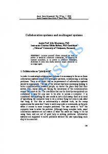
We conducted a series of parallel experiments with physical robots and in simulation. Our experimental testbed models the interior of a building, with a large space including six rooms and a “hallway,” which the robots explore, as described above. The physical arena is shown in Figure 3. We designed and implemented a dual system architecture, illustrated in Figure 1, in which both environments share common underlying system components. These include: a Task Allocator,

Task Allocator Stage Simulator

Camera Agent

Camera Agent

Camera Agent

Central Server

physical robots in arena

Robot Controller Robot Controller Robot Controller

Camera Agent

Camera Agent

Camera Agent

Fig. 1. Dual system architecture

a Central Server, and one Robot Controller for each robot. This dual architecture supports parallel experimentation and evaluation in both physical and simulation environments, such as those described in Section 5. The Central Server handles communication between system components, acting as a clearinghouse for passing messages. For each (physical or simulated) robot in the system, a Robot Controller is instantiated; it sends low-level messages to the robot about how to move. The details of our framework have been described elsewhere [36]. For now, it suffices to say that the framework is opensource and uses Player/Stage 6 [37, 38] as a hardware abstraction layer. The uniform API that Player provides allows us to write one controller for each kind of robot; this controller can communicate with either the physical platform or its simulated counterpart. (These are the boxes labeled “Robot Controller” in Figure 1.) The Task Allocator determines which robot should explore which interest point(s). For the work discussed here, only one allocation mechanism was used, but ongoing related work involves assessment and comparison of a range of different allocation mechanisms. The remainder of this section describes the differences between the physical and simulated environments. 4.1

Physical environment

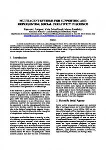
The two main components of the physical environment are the robots and a global vision system. Robots. Our multi-robot team is comprised of inexpensive, limited-function platforms. For the experiments described here, we used the Surveyor SRV-1 Blackfin,7 a small tracked platform equipped with a webcam and 802.11 wireless. Because the Blackfin (pictured in Figure 2) has very limited on-board processing, our robots rely on off-board processing. Each platform is wirelessly tethered to 6 7

http://playerstage.sourceforge.net/ http://www.surveyor.com/SRV_info.html

(a) unmodified

(b) with hat

(c) Braille hats

Fig. 2. The Surveyor SRV-1 Blackfin

a remote machine that runs its Robot Controller (as shown in Figure 1). This mode of communication naturally introduces some lag into the control loop. The global vision system (described below), however, makes the lag less pronounced than it would be if the robots relied on on-board vision, which would require the transmission of image data to the off-board robot controller. Global vision system. To provide an overhead view of the testbed, six Logitech C600 Webcams are suspended 10 feet above the arena. The cameras are arranged in a 2×3 grid, so each camera covers one sixth of the rectangular arena. Each camera is managed by a Camera Agent that employs OpenCV libraries8 [39] to handle image processing. The Camera Agents identify the robots and transmit their positions (2-dimensional location in global (x, y) arena coordinates and orientation θ, in degrees) to the Central Server. The Camera Agents function independently and only broadcast data to the Central Server; they do not receive any messages (other than acknowledgements that their own messages have been received). Since the robots are identical, the vision system needs some help to identify them uniquely. To distinguish among them, each robot is topped by a hat, a 4.25” by 5.5”,white rectangle with a pattern of 1.125” diameter black dots. The dots are arranged in a 2 × 3 grid; each grid square either has a dot or does not. Each hat is a character from the Braille alphabet9 . Examples appear in Figure 2. 4.2

Simulation environment

To support our simulation experiments, we employ the Stage environment that is integrated with Player. We can use Stage to run simulation experiments with exactly the same Robot Controllers used in the experiments with physical robots. The only difference is that rather than communicate with real robots in the test arena, in the simulation experiments, the Robot Controllers communicate with simulated robots in a Stage version of the test arena. 8 9

http://opencv.willowgarage.com/wiki/ http://www.afb.org/section.asp?SectionID=6

Fig. 3. The robots’ physical environment id operating starting number of mode configuration interest points PC3 physical clustered 3 PD3 physical distributed 3 PC8 physical clustered 8 PD8 physical distributed 8 SC3 simulated clustered 3 SD3 simulated distributed 3 SC8 simulated clustered 8 SD8 simulated distributed 8 Table 1. A summary of the experiments. For each, we conducted 5 iterations in the physical environment and 5 iterations in simulation.

5

Experiments and Results

As described in Section 3, our principal aim here is to compare the results obtained in simulation to those obtained with physical robots. Our experiments varied settings for three parameters: – operating mode: physical (P) or simulated (S); – initial conditions: starting positions for the robots that were distributed (D) or clustered together (C); and – number of tasks: number of interest points to allocate (m ∈ {3, 8}). For all the experiments described here, we used n = 3 robots. For each value of m tested, the interest points were in the same locations in the arena. There were two initial locations for the robots: clustered and distributed. Under clustered, the robots begin grouped together in the same “room” in the arena. Under distributed, the robots are spread into different rooms throughout

the arena. The clustered setting models the situation where the robots have just entered the space together. For example, an urban search and rescue scenario may have only one entry, through a doorway that is accessible to first-responders outside; it is quite reasonable that there would be only one such point. The distributed setting models the situation after some previous activity (e.g., mapping) has dispersed the robots. In both distributed and clustered settings, each robot starts from the same position for each run of the experiment (i.e., a given robot has a specific, repeated starting position for all the runs in an experiment on m tasks). The full set of combinations of parameters appears in Table 1. For each run of each experiment, we recorded the following measurements: – deliberation time, the total time required to allocate the tasks – execution time, the total time required to complete all the tasks and, for each robot, – travel velocity, the total distance it traveled divided by the amount of time that it was moving – idle time, the total amount of time that it was not executing a task, for example because it had no more interest points to visit – delay time time spent avoiding collisions with another robot, explained below Because each experiment involves many robots moving in a restricted area, they naturally get in each other’s way. When robots are close enough to require evasive action, our system detects a “near collision,” and the robots stop moving. Then the robot closest to its goal (current interest point) is given the right-of-way. The other robot waits until its path is clear, and then continues on its way. The time that a robot was stopped for this reason is its delay time. In addition to measuring delay time, we counted the number of times that robots were delayed in this manner (number of avoided collisions). 5.1

Results

The results reported here are based on five representative runs for each set of experimental conditions in the physical environment and for each set of experimental conditions in the simulated environment. Each experiment has a 3-character identifier: the first indicates the operating mode (P for physical and S for simulated); the second indicates the initial condition (C for clustered all in one room and D for distributed); and the third indicates the number of interest points in the problem (m ∈ {3, 8}). When we compare the results from the physical and simulated experiments under common conditions, we use the last two (common) characters of the identifier; for example, the results labelled C3 show the results for the experiments that used the clustered starting condition and sought 3 interest points. We compare the data in several ways. First, we compare the six numeric metrics described at the end of the previous section (deliberation time, execution time, travel velocity, idle time, delay time, and number of avoided collisions).

deliberation execution travel idle delay avoided time time velocity time time collisions PC3 0.99 (0.04) 89.89 (15.55) 10.54 (1.68) 80.34 (34.17) 19.18 (4.95) 8.2 (1.5) PC8 3.69 (0.43) 168.19 (41.15) 9.79 (2.00) 100.10 (51.79) 23.50 (7.84) 8.2 (3.5) PD3 1.18 (0.03) 58.64 (4.96) 12.99 (1.69) 23.33 (6.60) 8.61 (6.30) 2.6 (1.5) PD8 4.28 (0.08) 75.31 (17.72) 11.50 (1.88) 33.72 (28.52) 9.27 (6.50) 1.8 (1.1) SC3 1.06 (0.06) 272.03 (37.50) 2.54 (0.54) 141.26 (29.32) 136.71 (75.86) 10.2 (3.4) SC8 4.39 (0.22) 457.94 (33.26) 2.75 (0.33) 212.63 (40.69) 114.86 (35.57) 11.8 (3.0) SD3 1.36 (0.09) 221.11 (5.31) 3.05 (0.19) 80.62 (6.87) 36.82 (17.56) 3.8 (2.0) SD8 4.46 (0.16) 240.15 (1.20) 2.79 (0.21) 45.28 (2.94) 38.18 (1.30) 2.2 (0.4) Table 2. Summary of experimental results. Mean (standard deviation) over 5 runs.

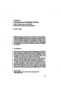
We compute the mean and population-based standard deviation for all metrics, averaged over the number of runs conducted for each set of conditions. A summary of those results appears in Table 2. The raw data is plotted in Figure 4. The second way we compare the results is by looking at the trajectories, or paths taken, by each robot. Sample trajectories are illustrated in Figure 5. The final way we consider the data is in terms of how well it supports our hypothesis and longer term goal, to use data collected in simulation as a predictor for data collected with physical robots. Analysis of Metrics. The first observation that we make about the results is that the metrics we collected are broadly in line with intuition, in the majority of cases. Our set of experiments covered two variables: problem size, as indicated by number of interest points, m ∈ {3, 8}; and starting condition, clustered or distributed. Thus, our expectations are as follows. First, we expect that metrics which measure the amount of time to compute and execute a solution will increase with problem size, i.e., deliberation time and execution time. Second, we expect that metrics which measure the amount of congestion the robots encounter when executing a solution will be larger when they start in a clustered setting, i.e., delay time and number of avoided collisions. Since the interest points themselves were distributed, we also expect that the robot usage will be more efficient when the robots start in a distributed setting; in other words, the total amount of time that robots who finish their tasks before others will sit “idle”, waiting for the others to finish, will be less than if robots start in a clustered setting—because in the latter case, some robots will have to travel further than others and the distance traveled by all robots will be more varied. These results match well. First, for all combinations of operating mode and initial conditions, deliberation time and execution time increase with problem size, as illustrated in Figures 4a and 4b, respectively. Second, the amount of idle time, delay time and the number of avoided collisions increases when robots start in the clustered setting, for both physical and simulated environments (Figures 4d, 4e and 4f, respectively).

5

500

4

400

3

300

2

200

1

100

0

0 C3

C8

D3

D8

C3

(a) Deliberation time

C8

D3

D8

(b) Execution time

20

300

250 15 200

10

150

100 5 50

0

0 C3

C8

D3

D8

C3

(c) Travel velocity

C8

D3

D8

(d) Idle time

300

20

250 15 200

150

10

100 5 50

0

0 C3

C8

D3

(e) Delay time

D8

C3

C8

D3

D8

(f) Number of avoided collisions

Fig. 4. A summary of the results. The experiment IDs describe the parameter settings. IDs are of the form hstarting conditionihnumber of robotsi: C indicates all the robots started clustered together, D indicates they were initially distributed. Results from all 5 runs conducted in each experimental condition are shown. The grey rectangles outline the range of results from the experiments conducted with physical robots. The unfilled rectangles outline the range of results from the experiments conducted in simulation.

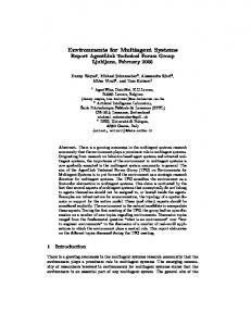
The travel velocity (Figure 4c) is slower in simulation, but this is because the simulator was not calibrated on the speed of the physical robots. In future work, we will calibrate the simulation to produce speed-up over the physical environment. However, the travel velocity data is still useful and in line with intuition, because it shows that the variation in speeds is much greater in the physical environment than in simulation. Path difference. The simulator does not capture the inaccuracies that dog the precise maneuvering of any robot. Compare Figures 5a to 5c and 5b to 5d to see this. These are traces of the position of the simulated and physical robots, respectively, in the D3 and C8 experiments. The fact that the simulator can still manage to produce reasonable predictions of some of our metrics led us to wonder how much the difference between the paths predicted by the simulator and those taken by the real robots might be affecting our results. Figure 5f attempts to assess this discrepancy. To obtain Figure 5f, we created a series of graphs like Figure 5e, which is the result of plotting a pair of paths from the same experimental scenario (where a given robot starts from a given point and ends at a given point); it treats the two paths as two sections of the perimeter of an oddly shaped polygon. The idea is that the area of this polygon is a measure of how much the paths differ from one another, where a larger area means more disparate paths. Once normalized by dividing the area by the perimeter, this produces an estimate of the difference between any two paths. On a pair of runs, this measures the variation between the two paths travelled. To assess a set of runs for a scenario, we took one of the runs of the physical robot and used the above method to compute how much that run varied from the other four runs of the real robots. For each of the four scenarios in Figure 5f, the average and standard deviation of this measure is plotted by the grey boxes. This same physical baseline run was then compared with the five simulated runs using the same method. These results are plotted in Figure 5f, where the clear boxes with the blue lines indicate the average value. The fact that these values are higher than their counterparts for the physical robots shows that the simulated runs are further from the baseline physical run than from the physical runs. In other words, the baseline physical run is more similar to the other physical runs than it is to the simulations. The physical runs also have a greater variance than the simulated runs, as one would expect. Once again, across the scenarios, the results from the simulations qualitatively match the results from the physical robots. Indeed, where the simulations suggest greater variation in path and thus a greater area, the performance of the physical robots bears this out. This suggests that despite the fact that the simulations do not predict the precise path taken by the real robots, they capture the essential features.

(a) SD3

(b) SC8

(c) PD3

(d) PC8 0.04 0.035 0.03 0.025 0.02 0.015 0.01 0.005 0 C3

(e) Path difference

C8

D3

D8

(f) Average path difference

Fig. 5. Comparing paths taken by simulated and physical robots. (a) and (c) simulated and real robot paths, respectively, for 3 interest points in the distributed scenario. (b) and (d) simulated and real robot paths, respectively, for 8 interest points in the clustered scenario. (e) An example of path difference (comparing the path of one robot in real and simulated versions of the 8-interest-point distributed scenario). (f) The average path difference across all scenarios.

Comparing the trajectory plots highlights some of the differences between the physical and simulation environments. Aside from the obvious disparities stemming from noise in the physical environment that is not present in the simulation, there is a difference between the two implementations regarding how a robot maintains its planned path during execution. In both environments, the path-planning algorithm uses A* to generate a sequence of multiple waypoints. To guide a robot from its current location to its next waypoint, its Robot Controller sends the robot a “goto” command, directing it to each point. This is translated into a “turn” followed by “go forward” commands sent to the robot platform (simulated or physical). A motion model is employed both in the simulation and the physical environment, to predict how far the robot travels given the commands it receives. In the simulation environment, we have perfect information about the position of the robot. The robot continually checks its position as it travels along its path, comparing its position as predicted by the motion model with its known (based on perfect information) position, and adjusts as necessary. In the physical environment, the robot’s position is computed by the global vision system or from a calibrated odometry model when the robot is not in the field-of-view of the vision system. The robot checks its predicted position with its computed position after completing the “goto” command. If it is not too far away from the desired waypoint, then the robot continues along to the next waypoint. If the robot has deviated significantly from the targeted waypoint, however, then it recalculates its path and generates a new set of waypoints from its current position to the nearest waypoint on the old path, resulting in a new, merged path that picks up from its current location and resumes with the path to the target interest point. The trajectories from the physical robot runs are characterized by much more jagged lines and paths than those of the simulated runs. This is due to two factors. First, the motion model in the physical environment, even though carefully calibrated for each robot platform, is more susceptible to noise, so the robot needs to adjust its path more frequently. Second, the global vision system is also susceptible to noise and produces noisy estimates of robots’ positions. If the position returned by the global vision system is significantly different from that estimated by the odometry model, then the vision estimate is ignored. In the trajectory plots for the physical robots, the dotted black lines (inside the colored paths) show the odometry estimates. Prediction. Finally, we examine how well our results support our hypothesis that the simulation can be a good predictor of our physical environment. Although we only executed a small number of runs within each experimental condition, we believe that the results can be used for predictions, as explained next. Our analysis of the raw data shows that most results are aligned in relative terms (e.g., execution time increases with problem size for both physical and simulation environments), though absolute numbers do not necessarily match. While the primary reason for lack of precise matching is due to the fact that the simulation does not mimic the clock time for robot motion, we actually do

not want the simulated robots to move at the same clock speed as the physical robots. Indeed, we would like the simulation to be able to run experiments more quickly than the physical environment, so that we can conduct more experiments in a shorter amount of time. So rather than seek precise matching of absolute numbers, we would like to see matching in relative, scaled terms. With this aim in mind, we re-examine our results, as illustrated in Figure 6. For each metric, we plot the range of the 20 data points collected across all 4 experimental conditions in the physical setting (4 conditions × 5 runs per condition). This range is illustrated by the height (y−range) of the grey-shaded boxes in the figure. Then we determine the range across all 20 data points collected in the simulated setting, and we scale these data to match the range of the physical data set. This scaled range is illustrated by the unfilled box to the right of each grey-shaded box: obviously, the heights of these boxes are the same as their left-hand-side counterparts. Then, we plot the mean and error bars (i.e., mean ± one standard deviation) for the metrics within each corresponding box. The simulated (sim) mean and standard deviation are scaled within the absolute range of the physical (phys) data: scaled sim value =

actual sim value − sim min × phys range + phys min sim range

where: phys range = (phys max − phys min) and sim range = (sim max − sim min) over all 20 data points collected in each environment. At least, we would like to see the scaled mean simulation values fall within one standard deviation of the (unscaled) physical data. At best, we would see the scaled error bars for the simulation values be completely contained within the error bars of the unscaled physical data. The “least” case holds for threequarters of the metrics: for 100% of values for execution time, for 75% of values for idle time, delay time and number of avoided collisions, for 50% of values for deliberation time and for 25% of values for travel time. The “best” case holds for only a few metrics: 50% for execution time and idle time, and none of the values for the other metrics. There are a number of cases where the opposite is true: the physical range falls completely within the scaled simulation range. Future work will investigate how we might improve the situation so that most metrics fall within the “best” case. One place to start is by examining the wider variation for some of the simulation metrics. Intuition says that there should be less variation in the non-physical environment, for example, with travel velocity. So we are examining the simulation environment to discern the cause of the variations.

5

250

4 200 3 150 2 100 1

0

50 C3

C8

D3

D8

C3

(a) Deliberation time

C8

D3

D8

(b) Execution time

18

200

16 150

14 12

100 10 8

50

6 4

0 C3

C8

D3

D8

C3

(c) Travel velocity

C8

D3

D8

(d) Idle time

40

15

30 10 20 5 10 0 0

-10

-5 C3

C8

D3

(e) Delay time

D8

C3

C8

D3

D8

(f) Number of avoided collisions

Fig. 6. Results plotted on a comparative scale. The experiment IDs describe the parameter settings. IDs are of the form hstarting conditionihnumber of robotsi: C indicates all the robots started clustered together, D indicates they were initially distributed. Mean and standard deviation computed over all 5 runs conducted in each experimental condition are shown. The grey rectangles outline the range of results from the experiments conducted with physical robots. The unfilled rectangles outline the scaled range of results from the experiments conducted in simulation. See text for more detailed explanation.

6

Summary and Future Work

This paper tests the hypothesis that metrics collected in simulation can be used to predict performance in a physical environment. In particular, we have investigated whether a simulated setting that runs exactly the same allocation mechanism and robot controller code can reliably predict properties that measure the performance of physical robots running in the real world. We tested this hypothesis in parallel experiments—running exactly the same tasks with both simulated and real robots, and measuring exactly the same metrics. Although the simulation does not predict the performance of every metric for every experiment, there is encouraging agreement at the qualitative level between the results obtained in simulation and those obtained with physical robots. We do not claim that our results will apply to all simulated/physical comparisons, but rather we make a case for making such comparisons in a systematic way and suggest metrics and analysis methods that produce promising results for our setting. Whether these metrics and methods will work for other settings is an open question. The work reported here is a first step towards a more ambitious and extended goal: the comparative evaluation of a broad range of coordination mechanisms from the multiagent literature implemented on physical multi-robot teams. Our future work is directed toward this goal. In particular, one of our next steps will be to adapt the current pseudo-auction mechanism so that bids take account of the whole path that a robot has to follow. Beyond that, we intend to investigate the performance of combinatorial auctions for this task allocation problem. In addition, we are also expanding our investigation of simulated-vs-physical settings by reviewing related work that addresses the same question and assessing the robustness of our methods and results in comparison with other studies. Acknowledgments This work was supported by the National Science Foundation under #CNS-0851901 and #CNS-0520989 and #IIS-1117000 and by CUNY Collaborative Incentive Research Grant #1642. The authors are grateful to Samuel Sanchez, Diquan Moore and Moses Kingston for their help in the development of the HRTeam framework. We would also like to thank anonymous reviewers of earlier versions of this paper for their helpful comments.

References 1. Jacoff, A., Messina, E., Evans, J.: A standard test course for urban search and rescue robots. In: Proc of the Performance Metrics for Intelligent Systems Workshop (PerMIS). (2000) 2. Murphy, R.R., Casper, J., Micire, M.: Potential tasks and research issues for mobile robots in robocup rescue. In: Robot Soccer World Cup IV, LNAI 2019, Springer Verlag (2001) 3. Habib, M.K.: Humanitarian Demining: Reality and the Challenge of Technology. Intl Journal of Advanced Robotic Systems 4(2) (2007)

4. Santana, P.F., Barata, J., Correia, L.: Sustainable Robots for Humanitarian Demining. Intl Journal of Advanced Robotic Systems 4(2) (2007) 5. D’Agostini, A., Calisi, D., an F. Fedi, A.L., Iocchi, L., Nardi, D.: Experimental Evaluation of Teamwork in Many-Robot Systems. In: Proceedings of Autonomous Agents and Multiagent Systems (AAMAS), Demonstration Paper. (2011) 6. Iocchi, L., Marchetti, L., Nardi, D.: Multi-Robot Patrolling with Coordinated Behaviours in Realistic Environments. In: Proceedings of the International Conference on Intelligent Robots and Systems (IROS). (2011) 7. Anderson, J., Baltes, J., Tu, K.Y.: Improving Robotics Competitions for RealWorld Evaluation of AI. In: Proceedings of the AAAI Spring Symposium on Experimental Design for Real-World Systems, AAAI Spring Symposium Series, Stanford, CA, USA (March 2009) 8. Cao, Y.U., Fukunaga, A.S., Kahng, A.B.: Cooperative mobile robotics: antecedents and directions. Autonomous Robots 4(1) (1997) 9. Lerman, K., Galstyan, A.: Mathematical model of foraging in a group of robots: Effect of interference. Autonomous Robots 13(2) (2002) 10. Williams, K., Burdick, J.: Multi-robot boundary coverage with plan revision. In: Proc of the IEEE Conference on Robotics and Automation. (2006) 11. Hollinger, G., Singh, S., Djugash, J., Kehagias, A.: Efficient multi-robot search for a moving target. Intl Journal of Robotics Research 28(2) (2009) 12. Parker, L.E.: Cooperative robotics for multi-target observation. Intelligent Automation and Soft Computing 5(1) (1999) 13. Murrieta-Cid, R., Muppirala, T., Sarmiento, A., Bhattacharya, S., Hutchinson, S.: Surveillance strategies for a pursuer with finite sensor range. Intl Journal of Robotics Research (2007) 14. Nerurkar, E.D., Roumeliotis, S.I., Martinelli, A.: Distributed maximum a posteriori estimation for multi-robot cooperative localization. In: Proc of the IEEE Intl Conference on Robotics and Automation. (2009) 15. Simmons, R., Apfelbaum, D., Burgard, W., Fox, D., Moor, M., Thrun, S., Younes, H.: Coordination for multi-robot exploration and mapping. In: Proc of the 17th National Conference on Artificial Intelligence. (2000) 16. Rooker, M.N., Birk, A.: Multi-robot exploration under the constraints of wireless networking. Control Engineering Practice 15 (2007) 17. Howard, A.: Multi-robot simultaneous localization and mapping using particle filters. Journal of Robotics Research 25(12) (2006) 18. Fox, D., Burgard, W., Kruppa, H., Thrun, S.: A probabilistic approach to collaborative multi-robot localization. Autonomous Robots 8(3) (2000) 19. Huang, G.P., Trawny, N., Mourikis, A.I., Roumeliotis, S.I.: On the consistency of multi-robot cooperative localization. In: Proc of Robotics: Science and Systems Conference. (2009) 20. LaValle, S.M., Hutchinson, S.A.: Optimal motion planning for multiple robots having independent goals. IEEE Transactions on Robotics and Automation 14(6) (1998) 21. Yamashita, A., Arai, T., Ota, J., Asama, H.: Motion planning of multiple mobile robots for cooperative manipulation and transportation. IEEE Transactions on Robotics and Automation 19(2) (2003) 22. Michael, N., Zavlanos, M.M., Kumar, V., Pappas, G.J.: Distributed multi-robot task assignment and formation control. In: Proc of the IEEE Intl Conference on Robotics and Automation. (2008)

23. Vail, D., Veloso, M.: Dynamic multi-robot coordination. In Schultz, A.C., Parker, L.E., Schneider, F.E., eds.: Multi-Robot Systems: From Swarms to Intelligent Automata. Kluwer (2003) 24. Gerkey, B.P., Matar´ıc, M.J.: Sold!: Auction methods for multi-robot control. IEEE Transactions on Robotics and Automation Special Issue on Multi-Robot Systems 18(5) (2002) 25. Koenig, S., Keskinocak, P., Tovey, C.: Progress on agent coordination with cooperative auctions. In: Proc of the AAAI Conference on Artificial Intelligence. (2010) 26. Lagoudakis, M., Markakis, V., Kempe, D., Keskinocak, P., Koenig, S., Kleywegt, A., Tovey, C., Meyerson, A., Jain, S.: Auction-based multi-robot routing. In: Proc of Robotics: Science and Systems Conference. (2005) 27. Dias, M.B., Zlot, R., Zinck, M., Stentz, A.: Robust multirobot coordination in dynamic environments. In: Proc of the IEEE Intl Conference on Robotics and Automation. (2004) 28. Gerkey, B.P., Matar´ıc, M.J.: A formal analysis and taxonomy of task allocation in multi-robot systems. Intl Journal of Robotics Research 23(9) (2004) 29. Zheng, X., Koenig, S.: K-swaps: Cooperative negotiation for solving task-allocation problems. In: Proc of the Intl Joint Conference on Artificial Intelligence. (2009) 30. Kalra, N., Ferguson, D., Stentz, A.: Hoplites: A market-based framework for complex tight coordination in multi-robot teams. In: Proc of the IEEE Intl Conference on Robotics and Automation. (2005) 31. Zlot, R., Stentz, A., Dias, M.B., Thayer, S.: Multi-robot exploration controlled by a market economy. In: Proc of the IEEE Conference on Robotics and Automation. (2002) 32. Frias-Martinez, V., Sklar, E.I., Parsons, S.: Exploring auction mechanisms for role assignment in teams of autonomous robots. In: Proc of the Eighth RoboCup Intl Symposium. (2004) 33. Hart, P., Nilsson, N., Raphael, B.: A formal basis for the heuristic determination of minimal cost paths. IEEE Transactions on Systems Science and Cybernetics 4(2) (1968) 34. Fujishim, Y., Leyton-Brown, K., Shoham, Y.: Taming the computational complexity of combinatorial auctions: Optimal and approximate approaches. In: Proceedings of the 16th International Joint Conference on Artificial Intelligence, Stockholm (1999) 35. Sandholm, T.: Algorithm for optimal winner determination in combinatorial auctions. Artificial Intelligence 135 (2002) 1–54 36. Sklar, E.I., Epstein, S.L., Parsons, S., Ozgelen, A.T., Munoz, J.P.: A framework in which robots and humans help each other. In: Proc of the AAAI Symposium Help Me Help You: Bridging the Gaps in Human-Agent Collaboration. (2011) 37. Gerkey, B., Vaughan, R.T., Howard, A.: The Player/Stage Project: Tools for MultiRobot and Distributed Sensor Systems. In: Proc of the 11th Intl Conference on Advanced Robotics (ICAR). (2003) 38. Vaughan, R.T., Gerkey, B.: Really Reusable Robot Code and the Player/Stage Project. In Brugali, D., ed.: Software Engineering for Experimental Robotics, Springer (2007) 39. Bradski, G., Kaehler, A.: Learning OpenCV: Computer Vision with the OpenCV Library. O’Reilly (2008)