May 5, 2006 - slope for which P had a complex-conjugate pair of isolated eigenvalues. ... it was proven that the location of a nontrivial real, positive isolated ... Figure 2: Largest 100 eigenvalues of an Ulam approximation of the ..... Pursuing this line of argument, we describe a numerical experiment for the map T from.
On Ulam approximation of the isolated spectrum and eigenfunctions of hyperbolic maps Gary Froyland∗ School of Mathematics The University of New South Wales Sydney NSW 2052, Australia May 5, 2006
Abstract Perron-Frobenius operators and their eigendecompositions are increasingly being used as tools of global analysis for higher dimensional systems. The numerical computation of large, isolated eigenvalues and their corresponding eigenfunctions can reveal important persistent structures such as almost-invariant sets, however, often little can be said rigorously about such calculations. We attempt to explain some of the numerically observed behaviour by constructing a hyperbolic map with a Perron-Frobenius operator whose eigendecomposition is representative of numerical calculations for hyperbolic systems. We explicitly construct an eigenfunction associated with an isolated eigenvalue and prove that a special form of Ulam’s method well approximates the isolated spectrum and eigenfunctions of this map.
Keywords: Perron-Frobenius operator, isolated spectrum, eigenfunction, almost-invariant set, Ulam’s method, hyperbolic map. 2000 Mathematics Subject Classification: 37M25, 37C30, 37D20.
1
Introduction
Perron-Frobenius operator (or transfer operator) methods are increasingly being used to solve problems arising in applications. Perron-Frobenius operators and their spectra have been very successful in the identification of molecular conformations [24]; transfer operators have enabled the detection of strange eigenmodes in fluid flow [21]; and Perron-Frobenius methods are being used to study the designs of office plans to ensure safe dispersal of airborne tracers such as smoke or radiation [20]. As Perron-Frobenius operators are a global representation of a system’s dynamics, their spectra and eigenfunctions provide powerful tools of global analysis. ∗
Work partially supported by UNSW Faculty of Science Research Grant PS06898.
1
Let T : M denote a discrete time dynamical system on a state space M , where for simplicity T is piecewise smooth and M ⊂ Rm . Denote by P : B(M ) , the Perron-Frobenius operator acting on a suitable space of real-valued functions (and distributions) on M . If B(M ) is carefully chosen, the spectrum of the Perron-Frobenius operator is contained in the unit disk, and of particular interest in applications are the eigenfunctions corresponding to the eigenvalue 1 and other real eigenvalues close to 1. Eigenfunctions of eigenvalues close to one represent slowly decaying modes. While at a microscopic scale, local expansion of T ensures rapid mixing, at a macroscopic scale, there are large structures determined by eigenfunctions corresponding to real eigenvalues close to 1 that persist for a very long time. These structures are known as almost-invariant sets [9, 13]. Quasi-compactness of the Perron-Frobenius operator has been proven in a variety of settings [23, 16, 22, 5, 14, 2]. Quasi-compactness of P : B(M ) allows for the existence of a nontrivial isolated1 spectrum, in particular, the existence of real eigenvalues close to 1. In the bounded variation setting, Baladi [1] produced an expanding Markov map of constant slope for which P had a complex-conjugate pair of isolated eigenvalues. In the same setting, Dellnitz et al. [8] described a parameterized family of expanding interval maps for which it was proven that the location of a nontrivial real, positive isolated eigenvalue may be controlled. For a C 2 expanding circle map, Keller and Rugh [17] proved the existence of an analytic eigenfunction for an isolated eigenvalue of P acting on C 1 test functions. In two-dimensions, Collet and Eckmann [7] construct a hyperbolic skew-product map with the expanding direction based upon the Baladi map [1], and show that Perron-Frobenius operator for this map inherits the complex-conjugate pair of eigenvalues from the one dimensional expanding dynamics. When one constructs Ulam discretizations2 [25, 19] of Perron-Frobenius operators of twodimensional (non-uniformly) hyperbolic maps, it is common for numerical eigenfunctions corresponding to non-unit eigenvalues to have the appearance of being smooth along (local) unstable fibres and very rough along (local) stable fibres. For example, the eigenfunctions corresponding to the largest subunit real numerical eigenvalues for (i) the Standard map and (ii) Arnold’s cat map are shown below in Figures 1 and 3.
This behaviour has also been
observed when, instead of discretizing via Ulam’s method, finite dimensional approximations are constructed by truncating a complete function basis. Weber et al. [26] demonstrate this ˜ = νh ˜ and |ν| is strictly larger than the essential spectral radius of We call ν an isolated eigenvalue if P h ˜ ˜ as an isolated eigenfunction of P. P for some nonzero h ∈ B(M ). We will refer to h 2 All Ulam matrices have been constructed using GAIO; http://www-math.unipaderborn.de/∼agdellnitz/gaio/. All eigenvalue and eigenvector calculations have been performed in MATLAB. 1
2
Figure 1: Ulam estimate of a “numerical eigenfunction” of the Perron-Frobenius operator of the Standard map S : T2 , S(x, y) = (x + y, y + 8 sin(x + y)) (mod 2π), corresponding to the numerical eigenvalue λ ≈ 0.7032 (based on a 256 × 256 grid).
effect for a kicked top on the sphere, creating a finite-dimensional representation of P by truncating a spherical harmonic basis of L2 ([−1, 1] × S 1 ). In order to better understand this behaviour, we construct a simple two-dimensional area preserving hyperbolic map that possesses a real, positive isolated eigenvalue. Moreover, we formally demonstrate that the corresponding eigenfunction has precisely the “smooth in unstable directions, rough in stable directions” behaviour that is numerically observed in many hyperbolic systems. We prove that Ulam’s method accurately approximates both this eigenvalue and the associated eigenfunction when the Ulam partition sets are adapted to the unstable and stable dynamics. The proof that Ulam’s method well approximates the isolated spectrum and eigenfunction relies upon the ability to separate the unstable and stable directions into two one-dimensional problems. Therefore, the method of proof does not easily generalise to arbitrary hyperbolic maps; indeed counterexamples to spectral stability of the pure Ulam method have been recorded [4, 5]. Nevertheless, this partial result is to our knowledge the first positive demonstration that a pure3 Ulam method can well approximate the isolated spectrum and eigenfunctions in a hyperbolic setting. The outline of this paper is as follows. In §2 we give an informal geometric description 3
Blank et al.[5] prove that one achieves convergence of the isolated spectra and associated eigenfunctions as the Ulam partition sets decrease in diameter provided that the action of P is smoothed by noise of the 1/3 order of (diameter of Ulam partition sets) . Unfortunately, Ulam’s method is almost exclusively applied in practice without such smoothing considerations as these would add considerably to the computational burden. Moreover, noise of this magnitude smooths away any fine structures in the eigenfunctions.
3
0.8 0.6 0.4 0.2 0 −0.2 −0.4 −0.6 −0.8 −1
−0.8
−0.6
−0.4
−0.2
0
0.2
0.4
0.6
0.8
1
Figure 2: Largest 100 eigenvalues of an Ulam approximation of the Perron-Frobenius operator of the Standard map, numerically estimated using a 256 × 256 grid. The eigenfunction associated with the largest subunit positive real eigenvalue λ ≈ 0.7032 is shown in Figure 1.
of the map. In §3 we demonstrate via a simple argument that the isolated spectrum of P contains 1/2. In §4 we construct the eigenfunction corresponding to 1/2 and in §5 we demonstrate that a specialised pure Ulam method with partitions aligned to unstable and stable directions well approximates the isolated spectrum (consisting only of 1/2 and 1) and the eigenfunction associated with 1/2. Numerical results and conclusions are presented in §6. Additional proofs are given in §7.
2
Geometric Description of an area preserving hyperbolic map
We begin with a geometrical description of our two-dimensional map T : [0, 1]2 of the unit square. The action of T is shown in Figures 5, 6, and 7. The unit square is compressed uniformly in the x-direction by a factor of four and expanded uniformly in the y-direction by a factor of four; see Figure 6. This long, thin rectangle is then divided into eight vertical strips which are reassembled to form a unit square; see Figure 7. The bijective map T is areapreserving and uniformly hyperbolic.
Because of the uniform expansion and compression
by a factor of four, one might expect that the mixing rate, or decay of linear correlation between two observables is geometric with rate 1/4. For many4 observables, we will verify that this is true. 4
more precisely, there is a co-dimension 1 subspace of observables which decay at an exponential rate at close to 1/4 or faster.
4
Figure 3: Ulam estimate of a “numerical eigenfunction” of the Perron-Frobenius operator of a smooth conjugacy of Anosov’s cat map C : T2 , C(x, y) = (2x + y, x + y) (mod 1), corresponding to the numerical eigenvalue λ ≈ 0.5538 + 0.01i (based on a 256 × 256 grid). For numerical stability in the eigenvalue computation, we have conjugated C with a diffeomorphism close to the identity.
However, note that the left half of the unit square is almost preserved under one application of T ; three-quarters of the left half remains in the left half. The same is true of the right half. Even though we have a stretching and compression of a factor of four at each iteration, there are some regions which do not mix at a rate commensurate with the local stretching. This behaviour can be explained by considering the eigendecomposition of the Perron-Frobenius operator of T .
3
Existence of an isolated eigenvalue
In this and the following section we define the Perron-Frobenius operator P (acting on suitable functions and distributions defined on [0, 1]2 ), demonstrate that P has an isolated ˜ : [0, 1]2 → R of P for this eigenvalue. eigenvalue 1/2, and construct an eigendistribution h Our Perron-Frobenius operator will act on a space of distributions that are smooth in the y-direction and rough in the x-direction. We use the functional analytic setup of [5]. The two main differences in settings between the present paper and [5] are firstly that we are working on the unit square rather than the 2-torus, and secondly that our space of regular functions used to define the distributions are allowed a discontinuity at x = 1/2. These two details are minor and are dealt with as required. Let 0 < β < γ ≤ 1. We introduce the set of functions Dβ which are β-H¨older in stable
5
0.8 0.6 0.4 0.2 0 −0.2 −0.4 −0.6 −0.8 −1
−0.8
−0.6
−0.4
−0.2
0
0.2
0.4
0.6
0.8
1
Figure 4: Largest 100 eigenvalues of an Ulam approximation of the Perron-Frobenius operator of Anosov’s cat map, numerically estimated using a 256 × 256 grid. The eigenfunction associated with the largest subunit “most positive” real eigenvalue λ ≈ 0.5538 + 0.01i is shown in Figure 3. Note that the numerics display no obvious isolated eigenvalue, consistent with the proof of an empty isolated spectrum for linear toral automorphisms; see Example 2.2.6 [5].
directions with H¨older constant 1, and with absolute value bounded by unity. Choose and fix some δ and define Dβ = {φ : [0, 1]2 → R : φ measurable, |φ|∞ ≤ 1, |φ(x1 , y) − φ(x2 , y)| ≤ |x1 − x2 |β for y ∈ [0, 1], |x1 − x2 | ≤ δ, x1 , x2 ∈ [0, 1/2) or x1 , x2 ∈ [1/2, 1]}.
(1)
This is the class of regular functions we will use to define our distributions. Note that the β-H¨olderness is measured only for x1 , x2 pairs in LHS and RHS of the unit square, allowing breaks in H¨older continuity across the line x = 1/2. For h ∈ C 1 ([0, 1]2 , R), and some fixed constant b > 0, let Z khks := sup hφ dm, φ∈Dβ [0,1]2 Z ∂h dm, khku := [0,1]2 ∂y khk := khku + bkhks , Z hφ dm, khkw := sup φ∈Dγ
(2) (3) (4) (5)
[0,1]2
where m is normalized Lebesgue measure on [0, 1]2 . The norm k · ks is a (weak) measure of roughness in the stable directions, while k · ku measures roughness in a stronger sense in the unstable direction. The norm k · k combines k · ks and k · ku , while k · kw is a weaker form of 6
1
7
8
5
6
3
4
1
2
0.75
0.5
0.25
0
0
0.5
1
Figure 5: Initial state of the unit square. 4
7 8
3
5 6
2
3 4
1
1 2
0
0 0.25
Figure 6: Intermediate state of the unit square under the action of T .
k · ks to be used for technical purposes. Let B([0, 1]2 ) and Bw ([0, 1]2 ) denote the completions of C 1 ([0, 1]2 , R) with respect to the norms k · k and k · kw respectively. The action of P on C 1 extends continuously to B([0, 1]2 ) and Bw ([0, 1]2 ). Lemma 1. B([0, 1]2 ) may be compactly embedded in Bw ([0, 1]2 ). This result is proven in Proposition 2.2.2 [5]. The setting here is slightly different as we work on a square instead of a 2-torus and Dβ allows breaks in β-H¨olderness at x = 1/2. The details of the proof of Proposition 2.2.2 [5] (in particular Lemma 3.6.2 [5]) can be followed through to check that Lemma 1 holds in the current setting. Proposition 1. P : B([0, 1]2 ) , is quasi-compact, and has an essential spectral radius bounded by 1/4β . Proof. Proposition 1 is almost an application of Theorem 1 [5]. Theorem 1 [5] applies to C 3 hyperbolic maps on T2 , while our example map T is only piecewise smooth and acts on [0, 1]2 . 7
1
0.9
0.8
0.7
0.6
0.5
3
1
5
8
7
4
2
6
0.4
0.3
0.2
0.1
0
0
0.125
0.25
0.375
0.5
0.625
0.75
0.875
1
Figure 7: Final state of the unit square under the action of T .
One needs to verify that the conclusion of Lemma 2.2.1 [5] holds; namely that a LasotaYorke inequality can be developed. Because of the uniform stretching and compression of the map T , verifying the existence of such an inequality is routine and we leave the details to the reader. Theorem 1 [5] states that the essential spectral radius of P is bounded by σ > max{1/4, 1/4β }. This yields the statement in Proposition 1. Theorem 1. For 1/2 < β < 1, P : B([0, 1]2 ) possesses an isolated eigenvalue 1/2. � R 1, if x < 1/2; 2 Then [0,1]2 h0 ·h0 ◦T n dm = Proof. Define h0 : [0, 1] → R by h0 (x, y) = −1, otherwise. n 1/2 , as the � action of T � on the sets {x < 1/2} and {x ≥ 1/2} is that of a Markov chain R 3/4 1/4 . Hence, [0,1]2 P n h0 · h0 dm = 1/2n . Let 1/4β < r < 1/2. Quasigoverned by 1/4 3/4 P compactness of P tells us that P n = ki=1 λni Πλi +Ψ, where λ1 , . . . , λk denote the eigenvalues
of P with moduli larger than r, Πλi denote the corresponding projections onto eigenspaces, R and kΨn k ≤ Hrn for some constant H > 0. Since [0,1]2 P n h0 · h0 dm = 1/2n and kΨn kw ≤ kΨn k ≤ Hrn , we must have that 1/2 = λi for some i = 1, . . . , k.
4
Construction of an isolated eigendistribution
One may obtain the eigendistribution of P corresponding to the isolated eigenvalue 1/2 via Π1/2 , the spectral projection for the eigenvalue 1/2. In this section, we construct this eigendistribution explicitly as the machinery we develop will be used in subsequent sections. Because our map is bijective and area preserving, the Perron-Frobenius operator may be written as Ph(x, y) = h(T −1 (x, y)).
8
(6)
The inverse of T is explicitly given by (4x, y/4), (4(x − 1/8), y/4 + 1/4), (4(x − 1/4), y/4 + 1/2), (4(x − 3/8) + 1/2, y/4 + 3/4), −1 T (x, y) = (4(x − 1/2), y/4 + 3/4), (4(x − 5/8) + 1/2, y/4), (4(x − 3/4) + 1/2, y/4 + 1/4), (4(x − 7/8) + 1/2, y/4 + 1/2),
x ∈ [0, 1/8); x ∈ [1/8, 1/4); x ∈ [1/4, 3/8); x ∈ [3/8, 1/2); x ∈ [1/2, 5/8); x ∈ [5/8, 3/4); x ∈ [3/4, 7/8); x ∈ [7/8, 1].
(7)
We will make use of the fact5 that
P(1(y)g(x)) = 1(y)g(Ts (x)), where Ts is the piecewise linear interval map defined below. 4x, x ∈ [0, 1/8); 4x − 1/2, x ∈ [1/8, 1/4); 4x − 1, x ∈ [1/4, 1/2); Ts (x) = 4x − 2, x ∈ [1/2, 3/4); 4x − 5/2, x ∈ [3/4, 7/8); 4x − 3, x ∈ [7/8, 1].
(8)
(9)
Let
Dβ,1 = {f : [0, 1] → R : f measurable, |f |∞ ≤ 1, |f (x1 ) − f (x2 )|/|x1 − x2 |β ≤ 1, x1 , x2 ∈ [0, 1/2) or x1 , x2 ∈ [1/2, 1]}. Introduce the norm kgks,1 = sup f ∈Dβ,1
Z
g · f dm.
(10)
Define B([0, 1]) to be the completion of C 1 ([0, 1]) with respect to k · ks,1 . Introduce the Koopman operator Us : B([0, 1]) , defined by Us g = g ◦ Ts for g ∈ C 1 ([0, 1], R), and the action of Us extended continuously to g ∈ B([0, 1]). Lemma 2. Define g0 : [0, 1] → R by ( 1, x ∈ [0, 1/2); g0 = −1, x ∈ [1/2, 1],
(11)
gn : [0, 1] → R by gn = 2n Usn g0 ,
(12)
and g˜ = limn→∞ gn . Then g˜ is a nonzero element of B([0, 1]) satisfying Us g˜ = g˜/2. 5
A similar observation is noted in [15], where eigenfunctions for the Perron-Frobenius operators of both the Bernoulli (circle-doubling) map and the standard Baker’s map are explicitly constructed in an L2 setting.
9
Proof. See proofs section. The graphs of g0 , g1 , and g2 are displayed in Figure 8. 1 g (x)
0.5 0
0 −0.5 −1 0
0.1
0.2
0.3
0.4
0.5 x
0.6
0.7
0.8
0.9
1
0
0.1
0.2
0.3
0.4
0.5 x
0.6
0.7
0.8
0.9
1
0
0.1
0.2
0.3
0.4
0.5 x
0.6
0.7
0.8
0.9
1
2
1
g (x)
1 0 −1 −2
4
2
g (x)
2 0 −2 −4
Figure 8: Graphs of g0 , g1 , g2 as labelled.
Theorem 2. Define gn as in (12). Under the conditions of Theorem 1, P : B([0, 1]2 ) pos˜ = limn→∞ hn sesses an isolated eigenvalue 1/2 and the corresponding eigendistribution is h where hn (x, y) = gn (x). Proof. The proof mimics the proof of Lemma 2. Using the norms (2), (3), and (4), we show ˜ = limn hn is a nonzero element of B([0, 1]2 ). To show that P h ˜ = h/2, ˜ that h we use the fact that kUs gn − gn /2ks,1 → 0 as n → ∞. By straightforward computation, P(hn (x, y)) = P(1(y)gn (x)) = 1(y)(Us gn (x)). Thus kPhn − hn /2k = k1(y)(Us gn (x)) − 1(y)gn (x)/2k = k1(y)(Us gn (x)) − 1(y)gn (x)/2ku + bk1(y)(Us gn (x)) − 1(y)gn (x)/2ks = 0 + bkUs gn (x) − gn (x)/2ks,1 → 0
5
as in the proof of Lemma 2.
Description of Ulam approximation
We construct via Ulam’s method a finite-dimensional approximation of the operator P : B([0, 1]2 ) . Typically, one constructs a sequence of partitions Pn = {A1 , . . . , AR(n) } of 10
[0, 1]2 comprised of regular partition sets with max1≤i≤R(n) diam(Ai ) → 0 as n → ∞. For a given n, an Ulam matrix Pn,ij = m(Ai ∩ T −1 Aj )/m(Ai ) and its left fixed eigenvector pn = PR(n) [pn,1 , . . . , pn,R(n) ] are computed, normalized so that i=1 pn,i = 1. In various settings [19, 11, PR(n) 10, 9, 5] one can show that the sequence of probability measures µn (B) := i=1 pn,i m(B ∩ Ai ) converges to an absolutely continuous or Sinai-Bowen-Ruelle measure. In the present
paper we make use of Ulam’s method to approximate eigenfunctions that are not fixed, but rather correspond to real eigenvalues close to 1. For piecewise smooth expanding interval maps without periodic turning points, Blank and Keller [4] show that the isolated spectrum is stable under certain stochastic perturbations, including the Ulam approximation. This work extended a similar result [3] for convolutiontype perturbations, which do not include Ulam-type approximations. In the two-dimensional Anosov setting, the author [12] demonstrated that if the Ulam matrix is constructed using a Markov partition, then Ulam’s method well approximated the isolated spectrum and the associated eigenfunctions of the induced expanding map on unstable foliations. In Theorem 3 below, for the map T from §2 we prove convergence of the eigenfunctions on the full space, not just on unstable foliations. In [5] a similar result is shown for reasonably general partitions when the Ulam construction is applied to a highly smoothed (relative to the partition sets) version of P. Theorem 3 uses a pure Ulam method, without smoothing. The map T described in §2 allows us to separate the unstable and stable dynamics. We prove convergence of the numerical estimates of the dominant subunit eigendistribution in the k · k norm. Our main result is: Theorem 3. Let {I1 , . . . , IP (n) } :=
Wn
k=0
Ts−k P0 where P0 = {[0, 1/8), [1/8, 2/8), . . . , [7/8, 1]}
and Ts is defined as in (9). Let {J1 , . . . , JQ(n) } be a partition of the unit interval. Partition the unit square via {Ip × Jq }p=1,...,P (n);q=1,...,Q(n) := {Ai }i=1,...,P (n)Q(n) . Assume that max1≤i≤P (n)Q(n) diam(Ai ) → 0 as n → ∞. Construct Pn,ij =
m(Ai ∩ T −1 Aj ) , m(Ai )
(13)
where m is normalised Lebesgue measure and T is defined as in §2. Compute the left ˆ n (x, y) := eigenvector vn corresponding to the eigenvalue 1/2 and construct the function h PP (n)Q(n) ˆ n (x) = hn (x), and thus h ˆ n → h, ˜ vn,i χAi (x, y). If vn is suitably normalised, then h i=1 ˜ are defined in Theorem 2. where hn and h Proof. See §7.
11
6
Numerical results and conclusions
We have constructed a hyperbolic map of the unit square whose Perron-Frobenius operator possesses an isolated eigenvalue. Further, we have proven that Ulam’s method, applied using a partition that is adapted to the stable and unstable directions successfully approximates both this isolated eigenvalue and its corresponding eigendistribution. Below we report on numerical calculations performed on a 128 × 128 grid P3 aligned to the coordinate axes. Figure 9 shows the largest 100 numerical eigenvalues of P3 . The numerical eigenvalue λ3 = 0.5108 approximates the eigenvalue 1/2, the existence of which was demonstrated in Theorem 1. ˆ 3 of the isolated eigendistribution h ˜ is shown in Figure 10. This numerThe Ulam estimate h 0.8 0.6 0.4 0.2 0 −0.2 −0.4 −0.6 −0.8 −1
−0.8
−0.6
−0.4
−0.2
0
0.2
0.4
0.6
0.8
1
Figure 9: Largest 100 eigenvalues of the Perron-Frobenius operator of the map T from §2, numerically estimated from an Ulam approximation on the 128 × 128 grid P3 . The numerical eigenfunction for the largest subunit positive real eigenvalue λ ≈ 0.5108 is shown in Figure 10. The small deviation of the numerically computed eigenvalue from 1/2 is due to numerical issues. Lebesgue measure is approximated by 961 sample points per grid set and the MATLAB eigenvalue routines have a finite accuracy tolerance.
ical eigenfunction very clearly displays the roughness in the stable direction and smoothness in the unstable direction discussed earlier. Moreover, Theorem 3 guarantees that the numerical eigenfunctions computed using Ulam’s method will converge in the k · k norm to the ˜ To our knowledge this is the first such positive proof that a pure isolated eigendistribution h. Ulam’s method can approximate the isolated spectrum and eigendistributions of hyperbolic maps on the full state space. Counterexamples to Ulam’s method reproducing the subunit spectrum have been reported in [4, 5] for Anosov’s cat map C. In [5] it is demonstrated that the Perron-Frobenius operator for C (acting on B(T2 )) has empty isolated spectrum, while [4, 5] detail a combina12
1 0.9 0.8 0.7 0.6 0.5 0.4 0.3 0.2 0.1 0
0
0.2
0.4
0.6
0.8
1
˜ of the Perron-Frobenius operator of Figure 10: Ulam estimate of the eigendistribution h T : [0, 1]2 as defined in §2, corresponding to the numerical eigenvalue λ ≈ 0.5108.
tion of theoretical and numerical evidence showing that Ulam matrices based upon several different partitions not aligned to the stable and unstable directions have large “fake” eigenvalues that � � lie outside the disk |z| ≤ 1/λu , where λu is the largest eigenvalue of the matrix 2 1 . In contrast, Brini et al. [6] demonstrate that for Anosov’s cat map, an Ulam ma1 1 trix based upon a Markov partition recovers the “correct” mixing rate of 1/λu . The strength of the counterexamples in [4, 5] is weakened by the fact [5] that the Perron-Frobenius operators of linear toral automorphisms do not have subunit isolated spectra to approximate when P acts on B(T2 ). One might argue that it is unreasonable to expect a finite-dimensional approximation such as Ulam’s method to correctly reproduce the non-isolated spectrum. Pursuing this line of argument, we describe a numerical experiment for the map T from §2, which we have shown does possess a subunit isolated eigenvalue. We conjugate T with C to obtain T˜ = C −1 ◦ T ◦ C. Using the partition P3 we compute the Ulam approximation P˜3 ˜ the Perron-Frobenius operator for T˜. As C preserves Lebesgue measure, P˜3 computed to P, on P3 equals P3 computed on the partition C(P3 ); this latter partition is now no longer aligned with the stable and unstable directions of T . Thus by computing P˜3 on P3 we achieve the effect of computing P3 on C(P3 ). The largest 100 eigenvalues of P˜3 are shown in Figure 11. The second largest eigenvalue of P˜3 is 0.4989, reproducing very well the eigenvalue 1/2 of P˜ (and P). Comparing Figures 9 and 11, we note that location of the third largest eigenvalue has moved outwards, but the second largest eigenvalue (in fact, in this case, the entire isolated spectrum of P) has remained relatively unchanged. Thus, while the isolated spectrum is well approximated, the spectral calculations in Figures 9 and 11 also 13
0.8 0.6 0.4 0.2 0 −0.2 −0.4 −0.6 −0.8 −1
−0.8
−0.6
−0.4
−0.2
0
0.2
0.4
0.6
0.8
1
Figure 11: Largest 100 eigenvalues of the Perron-Frobenius operator of T˜ = C −1 ◦ T ◦ C, numerically estimated from an Ulam approximation on the 128 × 128 grid P3 . The numerical eigenfunction for the largest subunit positive real eigenvalue λ ≈ 0.4989 is shown in Figure 10. The small deviation of the numerically computed eigenvalue from 1/2 is due to numerical issues. Lebesgue measure is approximated by 961 sample points per grid set and the MATLAB eigenvalue routines have a finite accuracy tolerance.
display the “fake” eigenvalues described in [4, 5]. This suggests that Ulam approximations accurately reproduce, at least in a partial sense, the non-isolated spectrum only in very special circumstances such as those outlined in [6]. ˜ = h/2, ˜ Turning now to the estimate of the isolated eigendistribution, since P h we have ˜ ◦ C) = (h ˜ ◦ C)/2. Thus we expect the eigendistribution h ˜ ◦ C to be smooth in directions ˜ h P( C −1 W u , where W u is the unstable direction for T , and rough in directions C −1 W s , where W s is the stable direction for T . These features are clearly seen in Figure 12. This experiment represents one positive example where it appears numerically that the subunit isolated spectrum and corresponding eigendistribution can be approximated by a pure Ulam’s method even when the partition sets are not adapted to the stable and unstable directions. Remark 1. An extension of property (8) is as follows. Call the Perron-Frobenius operator of a map of the unit square (F, G)-separable if there are piecewise smooth maps Tu , Ts : [0, 1] such that Pu is the Perron-Frobenius operator of Tu and Us is the Koopman operator of Ts and P(f (y)g(x)) = (Pu f )(y)(Us g)(x)
(14)
for f ∈ F ⊂ L1 ([0, 1], m) and g ∈ G ⊂ B([0, 1]) For example, the map T from §2 is (F, G)-separable for G = B([0, 1]) and F = {f ∈ L1 : f (y) = f (y + 1/4), 0 ≤ y < 3/4}. Approximation results such as Theorem 3 might be constructed for isolated eigendistributions 14
1 0.9 0.8 0.7 0.6 0.5 0.4 0.3 0.2 0.1 0
0
0.2
0.4
0.6
0.8
1
Figure 12: Ulam estimate of an eigenfunction of the Perron-Frobenius operator of T˜ = C −1 ◦ T ◦ C, corresponding to the numerical eigenvalue λ ≈ 0.4989.
h(x, y) = f (y)g(x) where f ∈ F, g ∈ G and P is (F, G) separable. As described in the introduction, Perron-Frobenius based numerical methods are increasingly being used in applications. Theorems 2 and 3 are a step towards formalising these calculations for multidimensional hyperbolic systems. While the piecewise smooth map T we have used clearly illustrates the features we wished to draw out, the question of whether there exists a smooth hyperbolic map with subunit isolated spectrum is to our knowledge still an open one. Extending Theorem 3 to more general partitions is very desirable, however the way forward is not clear and the existence of examples that have poor approximation properties makes it likely that a careful selection of hypotheses will be required to guarantee a positive result for a pure Ulam’s method. Despite these difficulties, we believe that a greater formal and numerical understanding of the information contained in the eigendecomposition of P can lead to powerful methods of analyzing global system properties.
7
Proofs
First, two technical lemmas. Lemma 3. Let f ∈ Dβ,1 and g ∈ B([0, 1]). Then
R
[0,1]
Us g · f dm =
R
[0,1]
g · Ps f dm
R Proof. g ∈ B([0, 1]) implies there is gm ∈ C 1 such that kgn −gm ks,1 → 0, that is, limm,n supf ∈Dβ,1 (gn · f − gm · f ) dm = 0. We define Us g via the limit of a smoothing of Us gm (we need to smooth
the Us gm as they are only piecewise C 1 ). For brevity, neglecting the smoothing, as it plays 15
no real role, Z
Us g · f dm := lim m
[0,1]
Z
gm ◦ Ts · f
[0,1]
Z
= lim gm · Ps f m [0,1] Z := g · Ps f
(see, for example, p.48 [18])
[0,1]
Lemma 4. kUs ks,1 = 1. Proof. We first prove that kUs ks,1 ≤ 1. kUs ks,1 =
sup
sup
g∈B([0,1]),kgks,1 ≤1 f ∈Dβ,1
=
sup
sup
g∈B([0,1]),kgks,1 ≤1 f ∈Dβ,1
≤
sup
sup
g∈B([0,1]),kgks,1 ≤1 f ∈Dβ,1
= 1
Z
Us g · f dm
(15)
[0,1]
Z
g · Ps f dm by Lemma 3,
[0,1]
Z
g · f dm
as Ps f ∈ Dβ,1 ,
[0,1]
By choosing g = f ≡ 1 in (15), we see that kUs ks,1 = 1. 1. To show g˜ ∈ B([0, 1]) is relatively straightforward. One may show
Proof of Lemma 2.
that standard C 1 smoothings of gn form a k·ks,1 -Cauchy sequence and by completeness, the limit g˜ ∈ B([0, 1]). 2. To show g˜ 6= 0 one may directly compute the limit of the norms kgn ks,1 and verify that this limit is 1. 3. To show Us g˜ = g˜/2, we demonstrate that kUs gn − gn /2ks,1 → 0 as n → ∞. We need to R show that limn→∞ supf ∈Dβ,1 [0,1] (Us gn (x)−gn (x)/2)f (x) dx = 0. First, some rewriting: Z lim sup (Us gn (x) − gn (x)/2)f (x) dx n→∞ f ∈D [0,1] β,1 Z (2n Usn+1 g0 (x) − 2n Usn g0 (x)/2)f (x) dx = lim sup n→∞ f ∈D [0,1] β,1 Z n = lim 2 sup (Us g0 (x) − g0 (x)/2)Psn f (x) dx by Lemma 3 (16) n→∞
f ∈Dβ,1
[0,1]
Let ¯ β,1 = {f : [0, 1] → R : f measurable, |f |∞ < ∞, |f (x1 ) − f (x2 )|/|x1 − x2 |β < ∞, D x1 , x2 ∈ [0, 1/2) or x1 , x2 ∈ [1/2, 1]}. 16
Define kf kβ,1 = |f |∞ + max{|f|[0,1/2] |β , |f|(1/2,1] |β }, where | · |β is the standard β-H¨older ¯ β,1 , k · kβ,1 ) , seminorm. It is relatively straightforward to demonstrate that Ps : (D the Perron-Frobenius operator for Ts , is quasi-compact with essential spectral radius bounded by 1/4β . Furthermore, the only spectral values outside |z| ≤ 4−β are 1/2 and 1, both with unit multiplicity. Thus we have the Ps -invariant decomposition ¯ β,1 = sp{1} ⊕ sp{g0 } ⊕ D ˜ β,1 , D ˜ β,1 corresponds to the essential spectrum. Thus any f ∈ D ¯ β,1 may be written where D ˜ β,1 and a1 (f ), a0 (f ), are uniquely determined. as f = a1 (f )1+a0 (f )g0 +f1 where f1 ∈ D R R As [0,1] gn dx = 0 for each n ≥ 0, without loss, we can assume that [0,1] f dx = 0;
thus a1 (f ) = 0. We demonstrate below that (16)=0 by separating the two cases. (a) f ∈ sp{g0 }: n
Z
lim 2 (Us g0 (x) − g0 (x)/2)2−n g0 (x) dx [0,1] Z = (Us g0 (x) − g0 (x)/2)g0 dx = 0
(16) =
n→∞
[0,1]
by direct computation. ˜ β,1 (b) f ∈ D (16) ≤ ≤ ≤
n
lim 2
n→∞
sup
Z
(Us g0 − g0 /2)kPsn |D˜β,1 kβ,1 f dx
˜ β,1 [0,1] f ∈D lim 2n kPsn |D˜β,1 kβ,1 n→∞
· kUs g0 − g0 /2ks,1
lim 2n · C · 4−βn (kUs ks,1 + 1/2)kg0 ks,1 = 0
n→∞
by Lemma 4
The remaining results are required for the proof of Proposition 2, stated later in this section. Let πn denote the canonical projection from B([0, 1]2 ) onto sp{χA1 , . . . , χAR(n) } defined by R(n)
πn h =
X i=1
1 m(Ai )
�Z
Ai
�
h dm χAi .
(17)
We describe the matrix representation of πn U on sp{χA1 , . . . , χAR(n) }. Lemma 5. Let {A1 , . . . , AR(n) } partition M ⊂ Rm and let U : L∞ (M, m) denote the Koopman operator for a Borel measurable map T : M . Then R(n) R(n) X X R(n) X m(Ai ∩ T −1 Aj ) χ Ai . πn U a i χ Ai = aj m(A ) i i=1 i=1 j=1
and under left multiplication the matrix representation of Un := πn U on the space sp{χA1 , . . . , χAR(n) } is Pn⊤ , where Pn is defined by (13). 17
The proof is included below for completeness; see Li [19] for the corresponding result for the Perron-Frobenius operator P. Proof.
R(n)
πn U
X i=1
R(n)
a i χ Ai = =
X
a i π n U χ Ai
R(n)
R(n)
X
1 m(Aj )
Z
R(n)
X
R(n)
X
X
1 m(Aj )
Z
i=1
ai
i=1
=
j=1
ai
i=1
j=1
R(n) R(n)
=
XX
ai
i=1 j=1
!
U χAi dm χAj
Aj
!
χT −1 Ai dm χAj
Aj
m(Aj ∩ T −1 Ai ) χ Aj m(Aj )
Interchanging i and j we have the result. For our particular interval map Ts defined in (9), we will compute left eigenvectors un of the matrix Un,s with eigenvalue 1/2 on the subspace sp{χI1 , . . . , χIP (n) }. The eigenvectors define piecewise constant functions which we show approximate the eigendistribution g˜ of Us in the k · ks,1 norm. Proposition 2. Let {I1 , . . . , IP (n) } = For each n, construct
Wn
k=0
Pn,s,ij =
Ts−k P0 where P0 = {[0, 1/8), [1/8, 2/8), . . . , [7/8, 1]}. m(Ii ∩ Ts−1 Ij ) m(Ii )
(18)
and compute the corresponding right eigenvector un for the eigenvalue λn = 1/2. Construct P the function gˆn (x) := nj=1 un,j χIj (x). If un is suitably normalised, then gˆn (x) = gn (x), and thus gˆn → g˜, where gn and g˜ are defined in Lemma 2.
Proof of Proposition 2. Construct an eight-symbol symbolic dynamics based on the partition P0 = {[0, 1/8), [1/8, 2/8), . . . , [7/8, 1]} := {I1 , I2 , . . . , I8 }. The topological dynamics induced by Ts on these subintervals is described by a subshift of finite type governed by the adjacency matrix
1 1 1 0 A= 1 0 0 0
1 1 1 0 1 0 0 0
1 1 1 0 1 0 0 0
1 1 1 0 1 0 0 0
0 0 0 1 0 1 1 1
18
0 0 0 1 0 1 1 1
0 0 0 1 0 1 1 1
0 0 0 1 . 0 1 1 1
(19)
As usual, let the cylinder [i0 · · · in ] denote the set Ii0 ∩ · · · ∩ Ts−n Iin . As in Lemma 2, define gn = 2n Usn g0 . Since gn (x) = 2n g0 (Tsn x), and Tsn ([i0 · · · in ]) = [in ], � n 2 , if x ∈ [i0 · · · in ] and in ∈ {1, 2, 3, 5}; gn (x) = n −2 , if x ∈ [i0 · · · in ] and in ∈ {4, 6, 7, 8}. Define un,i := gn (x) for x ∈ [(i − 1)/(2 × 4n ), i/(2 × 4n )), i = 1, . . . , 2 × 4n . We now show that un is a left eigenvector of Un,s . Each index i = 1, . . . , 2 × 4n represents a cylinder set of length n + 1. Consider the cylinder [i0 · · · in ]. Then with a slight abuse of notation, (un Un,s )[i0 ···in ] =
X
un,[i1 ···in a] /4.
(20)
a∈{1,...,8},Ain a =1
There are two cases to consider: firstly, in ∈ {1, 2, 3, 5}, so that three of the allowed un,[i1 ···in a] equal 2n and the remaining one equals −2n ; in this case, the sum (20) is 2n−1 , namely un,[i0 ···in ] /2; secondly, in ∈ {4, 6, 7, 8}, so that three of the allowed un,[i1 ···in a] equal −2n and the remaining one equals 2n ; again in this case, the sum (20) is −2n−1 , namely un,[i0 ···in ] /2. Thus, we have shown that un Un,s = un /2, and so gˆn = gn . By Lemma 2, kˆ gn − g˜ks,1 → 0.
We can now prove Theorem 3. Proof of Theorem 3. Consider the partition {I1 , . . . , IP (n) } of [0,1] from Theorem 3. By P Proposition 2, we have a sequence of eigenvectors un and step functions gˆn (x) = ni=1 un,i χIi (x)
satisfying gˆn → g˜ ∈ B([0, 1]). Now
πn P(1(y) · gˆn (x)) = πn (1(y) · Us gˆn (x))
by (8)
= 1(y) · πns (Us gˆn ) = 1(y) · gˆn (x)/2, ˆ n (x, y) := 1(y) · gˆn (x) is where πns is the canonical projection onto sp{χI1 , . . . , χIP (n) }. So h ˆ n − hk ˜ = k1 · gˆn − 1 · g˜k = an eigenfunction of πn P with eigenvalue 1/2. By Proposition 2 kh bkˆ gn − g˜ks,1 → 0.
8
Acknowledgements
The author is grateful to an anonymous referee for pointing out a simpler approach to proving Theorem 1 in an earlier version of this manuscript, and for discussions with Rua Murray. He thanks Mirko Hessel-von Molo, Oliver Junge, Kathrin Padberg, Stefan Sertl, and Bianca Thiere for assistance with GAIO.
19
References [1] Viviane Baladi. Unpublished, 1989. [2] Viviane Baladi and Masato Tsujii. Anisotropic H¨ older and Sobolev spaces for hyperbolic diffeomorphisms. Preprint, 2005. [3] Viviane Baladi and Lai-Sang Young. On the spectra of randomly perturbed expanding maps. Communications in Mathematical Physics, 156(2):355–385, 1993. [4] Michael Blank and Gerhard Keller. Random perturbations of chaotic dynamical systems: stability of the spectrum. Nonlinearity, 11:1351–1365, 1998. [5] Michael Blank, Gerhard Keller, and Carlangelo Liverani. Ruelle-Perron-Frobenius spectrum for Anosov maps. Nonlinearity, 15:1905–1973, 2002. [6] F. Brini, S. Siboni, G. Turchetti, and S. Vaienti. Decay of correlations for the automorphism of the torus T2 . Nonlinearity, pages 1257–1268, 1997. [7] P. Collet and J.-P. Eckmann. Liapunov multipliers and decay of correlations in dynamical systems. Journal of Statistical Physics, 115(1/2):217–253, 2004. [8] Michael Dellnitz, Gary Froyland, and Stefan Sertl. On the isolated spectrum of the PerronFrobenius operator. Nonlinearity, 13:1171–1188, 2000. [9] Michael Dellnitz and Oliver Junge. On the approximation of complicated dynamical behaviour. SIAM Journal for Numerical Analysis, 36(2):491–515, 1999. [10] Jiu Ding and Aihui Zhou. Finite approximations of Frobenius-Perron operators. a solution of Ulam’s conjecture to multi-dimensional transformations. Physica D, 92(1–2):61–68, 1996. [11] Gary Froyland. Finite approximation of Sinai-Bowen-Ruelle measures for Anosov systems in two dimensions. Random and Computational Dynamics, 3(4):251–263, 1995. [12] Gary Froyland. Computer-assisted bounds for the rate of decay of correlations. Communications in Mathematical Physics, 189:237–257, 1997. [13] Gary Froyland and Michael Dellnitz. Detecting and locating near-optimal almost-invariant sets and cycles. SIAM J. Sci. Comput., 24(6):1839–1863, 2003. [14] S´ebastien Gou¨ezel and Carlangelo Liverani. Banach spaces adapted to Anosov systems. Ergodic Theory and Dynamical Systems, 26:189–217, 2006. [15] Hiroshi Hasegawa and William Saphir. Unitarity and irreversibility in chaotic systems. Physical Review A, 46(12):7401–7423, 1992. [16] Franz Hofbauer and Gerhard Keller. Ergodic properties of invariant measures for piecewise monotonic transformations. Mathematische Zeitschrift, 180:119–140, 1982. [17] Gerhard Keller and Hans Henrik Rugh. Eigenfunctions for smooth expanding circle maps. Nonlinearity, 17:1723–1730, 2004. [18] Andrzej Lasota and Michael C. Mackey. Chaos, Fractals, and Noise: Stochastic Aspects of Dynamics, volume 97 of Applied Mathematical Sciences. Springer-Verlag, New York, 2 edition, 1994. [19] Tien-Yien Li. Finite approximation for the Frobenius-Perron operator. a solution to Ulam’s conjecture. Journal of Approximation Theory, 17:177–186, 1976.
20
[20] Prashant Mehta. Personal communication, 2005. [21] A. Pikovsky and O. Popovych. Persistent patterns in deterministic mixing flows. Europhys. Lett., 61(5):625–631, 2003. [22] David Ruelle. The thermodynamic formalism for expanding maps. Commun.Math. Phys., 125:239–262, 1989. [23] Marek Rychlik. Bounded variation and invariant measures. Studia Mathematica, 76:69–80, 1983. [24] Christof Sch¨ utte, Wilhelm Huisinga, and Peter Deuflhard. Transfer operator approach to conformational dynamics in biomolecular systems. In Bernold Fiedler, editor, Ergodic Theory, Analysis, and Efficient Simulation of Dynamical Systems, pages 191–223. Springer, Berlin, 2001. [25] S. Ulam. Problems in Modern Mathematics. Interscience, 1964. [26] Joachim Weber, Fritz Haake, Petr A Braun, Christopher Manderfeld, and Petr Seba. Resonances of the Frobenius-Perron operator for a Hamiltonian map with a mixed phase space. Journal of Physics A, 34:7195–7211, 2001.
21