Zineb Noumir, Paul Honeine. Institut Charles Delaunay (CNRS). Université de technologie de Troyes. 10010 Troyes, France. Cédric Richard. Laboratoire H.
ONE-CLASS MACHINES BASED ON THE COHERENCE CRITERION C´edric Richard
Zineb Noumir, Paul Honeine Institut Charles Delaunay (CNRS) Universit´e de technologie de Troyes 10010 Troyes, France ABSTRACT The one-class classification problem is often addressed by solving a constrained quadratic optimization problem, in the same spirit as support vector machines. In this paper, we derive a novel one-class classification approach, by investigating an original sparsification criterion. This criterion, known as the coherence criterion, is based on a fundamental quantity that describes the behavior of dictionaries in sparse approximation problems. The proposed framework allows us to derive new theoretical results. We associate the coherence criterion with a one-class classification algorithm by solving a least-squares optimization problem. We also provide an adaptive updating scheme. Experiments are conducted on real datasets and time series, illustrating the relevance of our approach to existing methods in both accuracy and computational efficiency. Index Terms— support vector machines, machine learning, kernel methods, one-class classification 1. INTRODUCTION In machine learning, several problems exhibit only a unique class for training. The decision rule consists of identifying if a new instance belongs to the learnt class or to an unknown class. This machine learning problem is the so-called oneclass classification problem [1, 2]. It has been applied with success for novelty detection, and extends naturally to tackle multiclass tasks by learning each class separately [3, 4]. Several methods have been developed to solve this problem, the most widely studied being the one-class support vector machines (SVM). It determines a sphere of minimum volume that encloses all (or most of) the training data, by estimating its center and radius. One-class SVM takes advantage of many properties from SVM literature, such as the nonlinear extension by using kernel functions and the sparse solution. The sparsity property states that the center of the sphere explores only a small fraction of the training samples, known as support vectors (SVs). A quadratic programming technique is often applied to solve this problem, i.e., identifying the SVs and estimating the optimal parameters. This work was supported by ANR-08-SECU-013-02 VigiRes’Eau.
Laboratoire H. Fizeau (CNRS) Universit´e de Nice Sophia-Antipolis 06108 Nice, France In this paper, we derive a one-class classification machine based on a new sparsification rule, the coherence criterion. This criterion is based on the coherence parameter, a fundamental quantity that describes the behavior of dictionaries in sparse approximation problems. We have recently investigated this sparsification criterion, and applied it with success in nonlinear filtering and online prediction in time series. See [5, 6]. The coherence criterion provides an elegant model reduction criterion with a low computational demanding procedure. This framework allows us to derive new theoretical results, mainly an upper bound on the error of approximating the center by the resulting reduced model. We associate the coherence criterion with a one-class classification algorithm by solving a least-squares optimization problem. We also provide an adaptive updating scheme for incrementing or decrementing the model order. The rest of the paper is organized as follows. Section 2 outlines the classical one-class SVM. We describe our approach in Section 3, by providing theoretical results and deriving an appropriate one-class classification algorithm. Section 4 provides an experimental study on real datasets and time series. 2. ONE-CLASS SVM Let x1 , x2 , . . . , xn be the set of training samples, et let Φ(·) be a nonlinear transformation defined by the use of a kernel, κ(xi , xj ) = !Φ(xi ), Φ(xj )". The one-class SVM finds a sphere, of minimum volume, containing all (or most of) the training samples. This sphere, described by its center c and its radius r, is obtained by solving the constrained optimization problem: n
min r2 + r,c,ζ
1 ! ζi νn i=1
subject to #Φ(xi ) − c#2 ≤ r2 + ζi for all i = 1, 2, . . . , n In this expression, ζ1 , ζ2 , . . . , ζn is a set of non-negative slack variables and ν a positive parameter that specifies the tradeoff between the sphere volume and the number of outliers, i.e., samples lying outside the sphere. By introducing the Karush-
(kernel) matrix, namely a µ-coherent set is1
Kuhn-Tucker optimality conditions, we get c=
n !
αi Φ(xi ),
µ = max |κ(xi , xj )|.
(1)
i,j∈I i"=j
i=1
where the αi ’s are the solution to the optimization problem: max α
subject to
n !
i=1 n ! i=1
αi κ(xi , xi ) −
n !
αi αj κ(xi , xj )
i,j=1
αi = 1 and 0 ≤ αi ≤
1 for all i = 1, 2, . . . , n. νn
It is well known that only a small fraction of the training samples contributes to the model (1). These samples, called support vectors (SVs), correspond to data outside or lying on the boundary of the sphere, and consequently contribute to the definition of the radius r. Thus, any new sample x that satisfies #Φ(x) − c# > r can be considered as an outlier, where the distance is ! ! #Φ(x)−c#2 = αi αj κ(xi , xj )−2 αi κ(xi , x)+κ(x, x), i,j∈I
i∈I
where I denotes the set of SVs, i.e., training samples with non-zero αi ’s. Let |I| denotes its cardinality. 3. PROPOSED ONE-CLASS METHOD
cn =
1 n
Φ(xi ).
(2)
i=1
We consider a sparse model of the center with ! cI = αi Φ(xi ),
Theorem 1. For the sparse solution cI satisfying the coherence criterion, the approximation error can be upper bounded with " #$ #cn − cI # ≤ 1 − |I|/n max κ(xi , xi ) − µ. (4) i
√ This upper bound takes the form (1 − |I|/n) 1 − µ for unitnorm kernels.
Proof. Let PI be the projection operator onto the space spanned by the elements Φ(xi ) for i ∈ I, thus cI = PI cn . Then, we have #cn − cI #
Let cn denotes the center of the n samples, namely n !
With the model order being fixed in advance, we consider the set of least coherence as the relevant set in the expansion (3). We have previously applied with success this coherence criterion in nonlinear filtering. See [5, 6]. In order to consider this sparsification rule for the one-class problem, one needs to study the relevance of the sparse model cI (obtained by the coherence criterion) with respect to the full-order center cn in (2). The following theorem provides a guarantee that this approximation error is upper bounded.
= ≤ =
n % %1 ! % % (1 − PI )Φ(xi )% % n i=1
n ! 1 #Φ(xi ) − PI Φ(xi )# n i=1 1! #Φ(xi ) − PI Φ(xi )# n i"∈I
(3)
i∈I
where the problem consists of properly identifying the subset I ⊂ {1, 2, . . . , n} and estimating the optimal coefficients αi ’s. While classical one-class SVM operates a joint optimization, we consider in this paper a separate optimization scheme: 1. Identify the most relevant samples in the expansion (3), by using the coherence parameter in the sparsification rule. 2. Estimate the optimal coefficients, with optimality in the least-squares sense, namely by minimizing #cn −cI #2 . 3.1. Sparsification rule with the coherence criterion The coherence of a set {Φ(xi ) | i ∈ I} is defined by the largest absolute value of the off-diagonal entries of the Gram
where the inequality is due to the generalized triangular inequality, and the last equality to the fact that #Φ(xi ) − PI Φ(xi )# = 0 for all Φ(xi ) belonging to the expansion in cI , i.e., for i ∈ I. Moreover, we have #Φ(xi ) − PI Φ(xi )#2 = #Φ(xi )#2 − #PΦ(xi )#2 & j∈I γj κ(xj , xi ) = κ(xi , xi ) − max & γ # j∈I γj Φ(xj )# ≤ κ(xi , xi ) − max k∈I
|κ(xk , xi )| κ(xk , xk )
≤ κ(xi , xi ) − µ where the first equality is due to the Pythagorian theorem, and the second equality follows the fact that the square norm of the projection of Φ(xi ) corresponds to the maximum 1 This definition corresponds to a unit-norm kernel, i.e., κ(x, x) = 1 ! for every x; otherwise, substitute κ(xi , xj )/ κ(xi , xi ) κ(xj , xj ) for κ(xi , xj ) in the expression.
iris ntrain |ntest class 0 25|125 class 1 25|125 class 2 25|125 mean: time: wine class 0 29|148 15.48 class 1 35|142 18.26 class 2 24|154 14.47 mean: 16.07 time: (22.2) cancer class 0 222|461 2.30 class 1 119|563 5.21 mean: 4.25 time: (42)
80% 70% 86% 79%
8.89 22.60 17.70 16.39 (0.3)
40% 46% 43%
3.03 4.78 3.90 (2.4)
8.57 7 16.51 13 12.81 13 12.63 11 (0.3) 2.12 3.80 2.96 (2.4)
9 8 8
Table 1. Experimental results with the classification error for each one-class classifier, and the mean error, as well as the total computational time (in seconds). The ratio of common SVs, with respect to the results obtained from the classical one-class SVM, for each of the proposed methods is given, as well as the mean ratio of common SVs. scalar product all the unit-norm functions ϕ, &!Φ(xi ), ϕ" over & namely ϕ = j∈I γj Φ(xj )/# j∈I γj Φ(xj )#. The first inequality results from a specific distribution of the coefficients, with γj = 0 for all j ∈ I except for a single index k with γk = ±1, depending on the sign of κ(xk , xi ). The last inequality follows from the coherence criterion.
3.2. Optimal parameters The coefficients are estimated by minimizing the approximation error #cn − cI #, namely n %1 ! %2 ! % % α = arg min % Φ(xi ) − αi Φ(xi )% , αi n i=1 i∈I
where α is a column vector of the optimal coefficients αk ’s for k ∈ I. Taking the derivative of this cost function with respect to each αk , and setting it to zero, we get
0.6
0.55
chlorine concentration
optimal this paper one-class same order as in order optimal from SVM optimal one-class SVM {3, 4, . . . , 15} error error shared SVs error |I| 1.84 0.49 50% 0.40 3 5.28 4.40 40% 1.28 4 4.80 4.10 60% 2.88 3 3.97 2.99 50% 1.52 3 (2.5) (0.6) (0.6)
0.5
0.45
0.4
0.35
0.3
0.25
1
2
Days
3
4
Fig. 1. Time series of the chlorine concentration, with one day for training (blue) and the next 3 days for error estimation (red). the need to operate from scratch as in SVM. For instance2 , one does not need to inversion the new Gram matrix. Let K −1 m be the Gram matrix defined on the set I with cardinality m. If one wishes to increment the model order to m + 1 by injecting the entry xk , then we have ' ( Km b K m+1 = b$ κ(xk , xk ) where b is the vector with entries κ(xk , xi ) for all i ∈ I. Then, the inverse of K m+1 can be computed using the block matrix inversion identity, with ' () ' ( * 1 −K −1 K −1 0 b −1 m m −b$ K −1 1 , K m+1 = + $ m 1 0 0 c (6) where c = κ(xk , xk )− b$ K −1 b and 0 is a m-length column m vector of zeros. The decremental update can be easily derived since, by using the notation ' ( Qm−1 q −1 Km = , q$ q0 $ we obtain from (6) the update K −1 m−1 = Qm−1 − qq /q0 .
4. EXPERIMENTATION
n
! 1! κ(xk , xi ) = αi κ(xk , xi ), for every k ∈ I. n i=1
Multiclass classification
i∈I
In matrix form, we obtain α = K −1 κ,
(5)
where K is the Gram (kernel) matrix, with entries κ(xi , xj ) for&i, j ∈ I and κ is a column vector with entries n 1 i=1 κ(xk , xi ) for k ∈ I. n An interesting property of the proposed method is that one can easily increment or decrement the model order, without
We have tested on three real datasets from the UCI machine learning repository, and well-known in the literature of oneclass machines [7]: “iris” with 150 samples in 3 classes and 4 features (only third and fourth features are often investigated), “wine” with 178 samples in 3 classes and 13 features, and “breast cancer” from Wisconsin with 683 samples in 2 classes and 9 features. 2 Updating expressions for the vectors α and κ can be easily derived, and were omitted due to space limitation.
In order to provide a comparative study, we considered the same configuration as in [8]. The Gaussian kernel was applied, with κ(xi , xj ) = exp(−#xi − xj #2 /2σ 2 ) where σ is the tunable bandwidth parameter. For an (-class classification task, a one-class classifier was constructed for each class, called target class. The target set was randomly partitioned into two subsets, one used for training and the other for the target test set. The whole test set contains the target test set and all the samples from the other classes. The classification error were estimated with the optimal parameters obtained by a ten-fold cross-validation on a grid search over ν ∈ {2−5 ; 2−4 ; · · · ; 24 ; 2−1.5 } and σ ∈ {2−5 ; 2−4 ; · · · ; 24 ; 25 }.
To compare the proposed method to one-class SVM (which is also comparable to [8]), we first considered the same number of SVs as in SVM. Table 1 gives the classification errors for both methods, as well as the ratio of shared SVs. We found that our approach is very competitive with the same model order as SVM, with up to 80% of common SVs. We also conducted a series of experiments to identify the optimal number of SVs for our algorithm, selected from {3, 4, . . . , 15}. This yields significant accuracy, as given in Table 1. The computational cost, using the best configuration of the tunable parameters, are given in terms of CPU time3 .
one-class SVM this paper
training error 8.90 % 0.20 %
time (m:ss) 1:16 0:02
coherence µ0 — 0.80
bound in (4) — 0.37
test error 63.7 % 1.9 %
Table 2. Results obtained for the time series problem. 5. CONCLUSION In this paper, we investigated a new one-class classification method, by using the coherence criterion. We derived an upper bound on the error of approximating the center of the sphere by the resulting reduced model. We incorporated this criterion into a new kernel-based one-class algorithm by solving a least-squares optimization problem, and considered an incremental and decremental schemes. Experiments were conducted on real datasets to compare our approach to existing methods. Perspectives include the use of this approach to derive an online one-class algorithm for novelty detection.
6. REFERENCES [1] D. Tax, “One-class classification,” PhD thesis, Delft University of Technology, Delft, June 2001.
Time series domain description We also conducted some experiments on a time series. It consists of the variation in chlorine concentration at a given node in a water network. Chlorine is a highly efficient disinfectant, injected in water supplies to kill residual bacteria. This time series exhibits large fluctuations due to the variations in water consumption and an inefficient control system. This data, taken from the public water supplies of the Cannes city in France, was sampled at the rate of a sample every 3 minutes. We considered 4 days of chlorine concentration measures. See Figure 1. To capture the structure of the time series, a 3-length sliding window was used, with xi = [xi−2 xi−1 xi ], where the Gaussian kernel was applied. Only the first day, that is 481 samples, was considered for training and estimating the optimal parameters using a 10-fold cross-validation configuration with σ ∈ {2−5 ; 2−4 ; · · · ; 24 ; 25 }. To be comparable with the one-class SVM, we considered |I| = 55 for both methods, obtained from ν = 0.004 in one-class SVM, leading to 60% of common SVs. Table 2 provides a comparative study, with training error given by the cross-validation, and the test error estimated on the next 3 days. This shows the relevance of our approach, where we also illustrate the upper bound on the approximation error derived in Theorem 1. 3 CPU time estimated on a Matlab running on a 2.53 GHz Intel Core 2 Duo processor and 2 GB RAM.
[2] B. Sch¨olkopf, J. C. Platt, J. Shawe-Taylor, A. J. Smola, and R. C. Williamson, “Estimating the support of a high-dimensional distribution.” Neural Computation, vol. 13, no. 7, pp. 1443–1471, 2001. [3] Y. Zhang, N. Meratnia, and P. Havinga, “Adaptive and online one-class support vector machine-based outlier detection techniques for wireless sensor networks,” in Proc. of the IEEE 23rd International Conference on Advanced Information Networking and Applications Workshops/Symposia, Bradford, United Kingdom, May 2009, pp. 990–995. [4] F. Ratle, M. Kanevski, A.-L. Terrettaz-Zufferey, P. Esseiva, and O. Ribaux, “A comparison of one-class classifiers for novelty detection in forensic case data,” in Proc. 8th international conference on Intelligent data engineering and automated learning. Berlin, Heidelberg: Springer-Verlag, 2007, pp. 67–76. [5] C. Richard, J. C. M. Bermudez, and P. Honeine, “Online prediction of time series data with kernels,” IEEE Transactions on Signal Processing, vol. 57, no. 3, pp. 1058–1067, March 2009. [6] P. Honeine, C. Richard, and J. C. M. Bermudez, “On-line nonlinear sparse approximation of functions,” in Proc. IEEE International Symposium on Information Theory, Nice, France, June 2007, pp. 956–960. [7] D. Wang, D. S. Yeung, and E. C. C. Tsang, “Structured one class classification,” IEEE Trans. on systems, Man, and Cybernetics, Part B, vol. 36, pp. 1283–1295, 2006. [8] Y.-H. Liu, Y.-C. Liu, and Y.-J. Chen, “Fast support vector data descriptions for novelty detection,” IEEE Trans. on Neural Networks, vol. 21, no. 8, pp. 1296–1313, aug. 2010.