... and strongest-neighbor approaches, the PDA is all-neighbors. 1 This work was supported by Center of Excellence BIS21 under the Grant ICA1-2000-70016 ...
One Particular Program Realisation of JPDA Algorithm1 L. V. Bojilov, K. M. Alexiev, P. D. Konstantinova Abstract. In JPDA-algorithm realisation, some particular problems have to be solved. They include clusterisation of the tracks, generation of all feasible hypotheses and optimisation of the numerical expressions for overcoming calculation drawbacks. These problems are not of theoretical importance. However, if they are not solved in a proper way, it will be very difficult to tailor a workable JPDA algorithm. We expose practically useful algorithms for the problems mentioned above and discuss a simple optimisation scheme for numerical expressions in the program. 1.Introduction. The Joint Probability Data Association (JPDA) algorithm is intended to deal with multiple targets in clutter, assuming dense target scenario [1,2]. This algorithm is a special case of the MHT method[2]. It is not so powerful as Multiple Hypotheses Tracking (MHT) approach, but it leads to much less computational load. When numerous targets present in surveillance region, there is no need to process all of them in the JPDA algorithm frame simultaneously. As a first step at a given scan, say k, all existing targets have to be divided into separate groups (clusters). Every such a group will contain tracks with overlapping validation gates and shared observations. In this way, the dimension of the task of JPDA algorithm will be equal to the number of the tracks in a given cluster. The next important step is hypotheses generation. Every hypothesis H l represents a particular way the measurements in a cluster are associated with the targets. In addition, for every hypothesis the probability P(H l ) of being true has to be calculated. Our attention to the hypotheses generation and probability calculation is due to the fact, that this is one of the most time consuming parts of the overall JPDA algorithm. In one of our numerical tests with four targets and ten observations in the cluster, the generated feasible hypotheses have reached the number of 378. It is obvious, that even in middle-sized problems the combinatorial explosion may overwhelm the calculations. In the next section we outline in brief the PDA algorithm and point out its extension to JPDA algorithm. The parts of the JPDA algorithm needed to be optimised are identified and the motivations for these efforts are discussed. In the third section all improvements of the JPDA algorithm are expressed and considered: the hypotheses generation; optimisation of the hypotheses’ probabilities computation; and heuristic formula for false targets density calculation. 2.Problem formulation. The PDA approach was first presented by Bar-Shalom and Tse [3]. In contrast to nearest-neighbor and strongest-neighbor approaches, the PDA is all-neighbors 1
This work was supported by Center of Excellence BIS21 under the Grant ICA1-2000-70016
1
approach. The PDA tracks targets by using the weighted average of the innovations of all measurements in the gate. Following
S.BLACKMAN
[2] The main steps of the algorithm can be
stated as follows: Assuming that false targets are presented and their probability density is β . Given N observations within the gate, there are
N+1
hypotheses that can be formed. The first
hypothesis (H 0 ) is the case in which none of the observations is valid. The probability of H 0 to be true is proportional to
(1)
p i′0 = β N (1 − PD )
The probability of the other hypotheses H j ( j = 1,2,� , N ) that observation j is a valid return is proportional to
(2)
p ij′ =
β N −1 PD e
(2π )M 2
−
d ij2 2
⋅
Si
Here d ij2 = ~ z ijT S −1 ~ z ij is squared normalised distance between observation j and target i , S is residual covariance matrix, β is spacial density for false measurements and PD is probabilty for target detection. At last, through normalization we compute the probabilities of all N+1 hypotheses:
(3)
pij =
pij′ N
∑ p′
⋅
il
l =0
This is the first main step of the algorithm. The next step is to compute the combined innovation of scan k for use in the Kalman filter update equation:
(4)
~z (k ) = ∑ pij ~zij (k ), where ~zij (k ) = z j (k ) − Hxˆ i (k k − 1)⋅ i N
j =1
The last step in the PDA algorithm include standard Kalman filter equations with the modified update equation for covariance P. This modification is intended to reflect the effect of uncertain correlation. The JPDA algorithm is an extension of the PDA method but for dealing with multiple targets. The only difference is the computation of the association probabilities of (3) by using all observations and all tracks in a cluster. The first step of this extension is clusterisation of all targets in the surveillance region. The typical example of such a cluster is shown in fig.1. All three tracks in the cluster are with overlapping validation regions and shared observations.
2
The next step of the JPDA extension is to generate all feasible hypotheses. Every feasible hypothesis, H l , represents a particular way the measurements in a given cluster have to be associated with the targets. The feasibility of the hypotheses requires that: •
Each target generates only one measurement (which may or may not be detected);
•
Each measurement corresponds to only one target.
The third step (of the JPDA extension) is to compute the probabilities of the generated feasible hypotheses. The multipliers in the expression for probabilities computation correspond to:
β - probability density for false returns, PD , (1 − PD ) - probability of target detection and target missing respectively, g ij =
e
−
d ij 2
(2π )M 2
- probability density that measurement j originates from target i. S
With some additional notations concerning one particular cluster N M - total number of measurements, N T - total number of targets, N F - number of false returns,
3
N nD - number of not detected targets, the common view of the probability expression will be
(5)
P′(H l ) = β [N M −( NT − N nD )] (1 − PD )
N nD
PD
( NT − N nD )
g ij � g mn ⋅
In the above expression, the number of multipliers g ij is equal to (N T − N nD ) . This step ends with standard normalisation
(6)
P(H l ) =
P′(H l ) NH
∑ P′(H )
, where N H is the total number of hypotheses.
l
l =1
The final step of the JPDA extension is association probability
computation. To
compute for a fixed i the probability pij that observation j originates from track i we have to take a sum over the probabilities of those hypotheses in which this event occurs: pij =
∑ P(H ) ,
l∈L j
l
where L j is a set of numbers of all hypotheses, which include the event, mentioned above. It is obvious that for a fixed i
(Lm ∩ Ln ) = 0
for indices of all measurements in the validation region
of target i . On the other hand, for a fixed i , all hypotheses will be included in computation of pij . Because of that and due to (6), the sum of probabilities pij for a fixed i adds up to unity. With this step the JPDA extension loop terminates and the algorithm continues with the computation of the combined innovations (4) of the standard PDA. 3.The JPDA program optimisation. The main drawback in JDPA algorithm implementation, in spite of all, is computational load, especially in the case of many closely spaced targets and big clusters and in the presense of clutter. Our efforts in this work are directed to optimisation of calculations in some points of the JPDA extension’s steps. Probability expression optimisation. Let’s to assume that N M > N T and to consider the expression (5). It can be rewritten as follows:
(7 )
[
P ′(H ) = β (N M − NT ) β N nD (1 − PD )
N nD
PD
( N T − N nD )
]
g ij � g mn ⋅
It can be easily seen that the factor out of the brackets is common factor appearing in all members of a sum in (6) and so, it will be cancelled. In view of this, we can miss this factor in (5) saving, in this way, redundant multiplications. In the opposite case, when N T > N M , the common factor will be (1 − PD )
(NT − N M )
and analogous operations can be performed.
4
A heuristic formula for false density calculation. Using the nonparametric PDA, one can replace the spatial density β with the expression of so called sample spatial density [4]:
β=
m(k ) , where m(k ) is the number of measurements in the validation region, V (k )
and V (k ) is the volume of this region. In the JPDA algorithm, however, there are several targets in the cluster with validation regions overlapped and with shared measurements. In this case, the sample spatial density will be expressed by:
β=
NM , where N M is the total number of measurements V1 (k ) ∪ V2 (k ) ∪ � ∪ V N c (k )
in the cluster and in the denominator is the total volume of all validation regions without duplicating the overlapping parts. To calculate the exact total volume of all targets in the cluster in practice is rather difficult. We propose here an easy to be calculated heuristic formula, which proved to be a good approximation of the above expression in many numerical experiments: NT
(8)
β=
∑ m (k ) i
i =1 NT
∑V (k ) i =1
⋅
i
The motivation of this formula is that we allow duplication of the overlapping parts in the denominator, but we allow duplication of the shared measurements in the numerator too. The numerical experiments confirm that the proposed formula is a good approximation of the sample spatial density. An algorithm unifying both hypotheses generation and hypotheses probability computation. An important and most time-consuming part of the JPDA algorithm is hypotheses generation and hypotheses probability computation. The proposed here algorithm computes hypothesis probability simultaneously with its generation. We will illustrate our idea by using an example. Table 1 sumarize the information describing scenario from fig 1. Table 1. Target 1 0 1
β (1 − PD ) PD g 11
Target 2
β (1 − PD ) PD g 23
0 3
2
PD g 12
4
PD g 24
3
PD g 13
5
PD g 25
5
Target 3 0 5 6
β (1 − PD ) PD g 35 PD g 36
Every target covers two columns. The first column contains the numbers of measurements falling in its validation region. The second column contains the multiplyers which have to be included in the optimized expression (7) when the target and the measurement are associated in corresponding hypothesis. For example, to list the first several hypotheses and their respective probabilities using Table 1:
0
0
0
-
β 2 (1 − PD )2 β (1 − PD ),
0
0
5
-
β 2 (1 − PD )2 PD g 35 ,
0
0
6
-
β 2 (1 − PD )2 PD g 36 ,
0
3
0
-
β (1 − PD )PD g 23 β (1 − PD ),
0
3
5
-
β (1 − PD )PD g 23 PD g 35 ,
0
3
6
-
β (1 − PD )PD g 23 PD g 36 .
It can be seen that the probabilities of every two hypotheses for the most inner cycle differ with one multiplier and we can compute every of these expressions by means of one multiplication only. For every new value of the index of upper next cycle an additional multiplication can be performed. So, a significant reduction of needed multiplications can be achieved in computing hypotheses probabilities, if construct an algorithm in which every time when index of the most inner cycle runs, the value computing up to this cycle to be saved unchanged. For estimating the reduction of calculations by implementing this idea to assume N groups (targets) of elements (measurements) with n1 , n 2 ,� , n N elements in every group. To assume too, that every possible combination is feasible. The scores (or probabilities) of all possible combinations can be computed by performing M = n1 , n 2 ,� , n N (N − 1) multiplications. If we use the mentioned above idea, however, a simple formula can be derived for needed number of multiplications: M ′ = n1 n2 (1 + n3 (1 + n4 (1 + � n N −1 (1 + n N )�))) ⋅ It can be noticed that M ′ reaches its minimum when groups are ordered so, that number of their elements monotonically increase. In order to estimate the reduction ratio we assume an additional simplification that the number of elements of all N groups is equal to n. After some simple transformations we obtain: M n −1 (N − 1)⋅ = M′ n
6
If we realize, for example, the case, when N = 5 and n = 5, the reduction ratio will be 3.2 and we can expect, that this value is lower bound in comparison with the most common case. Let us consider the case when in five groups (N=5) the number of elements are 3, 4, 5, 6 and 7 respectively. The common number of elements in all five groups will be the same, as in the previous case, but reduction ratio will be now equal to 3.4. The most easily, this algorithm can be implement as a recursion. 4.Numerical results. In order to verify our ideas we have carried out a series of numerical experiments with program realization of the described above algorithm. We construct a typical scenario for targets’ motion, including five targets moving along five parallel and closely spaced trajectories(fig.2). In the beginning of the process targets are so separated that their validation regions do not overlap. The most appropriate model of the number of false alarms in a volume V is given by binomial distribution N N −m P(m ) = p m (1 − p ) , m where N is number of resolution cells in this volume an p is probability of false alarm in each cell. But in view of computational difficulties more suitable model is Poisson distribution which is known to be a good aproximation of binomial distribution when p (or 1-p) is less then 0.1[4]: P ( m ) = e − βV
(βV )m . m!
Here the Poisson parameter β is the sample spatial density, defined as β =
m . V
Because of the different velocities the five targets become moving closer end validation regions of some of them become overlapped. If in the overlapped volume fall a measurement the corresponding targets form a cluster. In the midle of the scenario more often four or five targets move in a cluster depending on randomly disposed false measurements. We perform two series of experiments with β = 1 and β = 2 respectively. Averaging over ten runs for every one value of β we derive the number of floating point operations per cluster with 2, 3, 4 and 5 targets each. The results are given in the table 2. Table 2. Floating point operations per cluster
β =1 Number of targets Nonoptimized in a cluster version 2 207 3 747
Optimized version 184 629
β =2 Reduction ratio 1.12 1.19
7
Nonoptimized version 229 2739
Optimized version 202 2189
Reduction ratio 1.14 1.25
β =1 4 5
7599 35333
β =2
5705 24290
1.33 1.45
14772 151360
10937 103598
1.35 1.47
Even more informative is table 3, where for the same frame of experiments the processing time (in seconds) is summarized and averaged for every type of cluster. Table 3. Processing time (in seconds) for every kind of cluster
β =1 Number of targets Nonoptimized in a cluster version 2 3 0.0225 4 0.423 5 4.5
β =2
Optimized version 0.0213 0.1 0.438
Reduction ratio 1.06 4.23 10.27
Nonoptimized version 0.068 0.51 38.1
Optimized version 0.0377 0.19 5.71
Reduction ratio 1.8 2.68 6.67
The results from the table confirm the dependence of processing time on number of targets in the cluster, which prove to be near to exponential. On the other side, processing time depends on the number of measurements in the gate too. It can be noticed, as well, that reduction ratios in table 3 are much more impressive than reduction ratios in table 2. The difference can be explain that proposed optimization assumes more effective program code. 5. Conclusions. In this appear some practical aspects of program realization of JPDA algorithm have been considered. Analyzing the algorithm steps three optimizations have been proposed. First end third optimization reduces the floating-point operations to be performed. Third optimization in addition enables more effective program code. The second optimization overcomes difficulty to compute the sample spatial density. Numerical experiments show that the proposed trade-off in computing this density does not lead to association probability degradation. As a result, the program realization of the JPDA algorithm demonstrates considerable speed up of its work and improved performance. REFERENCES: [ 1]
BAR-SHALOM, Y., THOMAS E. FORTHMANN,
Academic Press, 1988; [2]
BLACKMAN S. S.,
Norwood, MA, Artech House, 1986; [3]
Tracking and Data Association, San Diego, CA,
Multiple-Target Tracking with Radar Applications,
BAR-SHALOM, Y., E. TSE,
Tracking in a cluttered
inveronment with probabilistic data association, Automatica, Vol. 11, Sept. 1975, pp 451-460. [4] BAR-SHALOM, Y.
and
XIAO-RONG
LI,
Multitarget-Multisensor Tracking: Principles and
Techniques, Storrs, CT, YBS Publishing, 1995;
8