Ongoing Experiments in Autonomous 2D Shape Formation, With A View to Developing Autonomous 3D Formations With Unmanned Dirigibles Ian Mudie, Chris Melhuish and Alan Winfield Intelligent Autonomous Systems Engineering Laboratory, University of the West of England, Coldharbour Lane, Bristol, BS16 1QY. E-mail:
[email protected] 2nd March 2001 Abstract: This paper reports on the preliminary simulation experiments that have been conducted in the search for a control system design that will allow an unknown number of autonomous dirigibles to manoeuvre into a pre defined three-dimensional formation.
1.0 Introduction In recent years, a large amount of research has been conducted into producing two and threedimensional flocking. This has been accomplished with wheeled robots by Kelly and Keating [1996] & Gulliford [1998], in simulation by Reynolds [1987], and Graves [1997], and with autonomous dirigibles by Welsby [2000]. Spatial self-organisation and team building has also been studied by Unsal & Bay [1994], and Sharman [1994]. The findings that are reported in this paper are part of an ongoing research project in developing a high level control system, along with the necessary hardware, that will allow an unknown quantity of unmanned dirigibles to produce a three dimensional formation. It is the author’s belief that this type of spatial self-organisation has not previously been attempted with dirigibles. In order to achieve this task the current dirigible hardware design includes equipment that allows for, the reception of orders, agent identification, agent alignment, and range finding. By adapting an idea from Arai et al. [1999], where a ring of infrared transmitters and receivers are used for obstacle avoidance, one possible method of achieving the above task is currently being developed. A computer simulation has been used to test how well the current behaviour based control system performs when instructed to produce line, square and cross-shaped formations. The simulated agents each possess eight sensor modules that are arranged around the circumference of the agent’s body. Each module contains wide and narrow angle infrared transmitters and receivers for identification and alignment, ultrasonic range-finding equipment for collision avoidance and spacing, and a radio frequency transceiver for receiving orders and passing on information. A behaviour based control system is employed, and was originally implemented with a subsumption like architecture [Brooks 1985]. This has since been changed for the purposes of simulation. This paper first describes the target platform for the developed control system. This has been decided upon with knowledge gained from previous dirigible research work, payload capacity and available sensor systems. The simulation models this hardware arrangement onto the agents, details of which can be found in section 2. Section 3 details the first experiment, which attempts to arrange the agents into a straight line. Section 4 reports on the results obtained when a square formation was attempted in experiment 2. Details of the final experiment, which attempts to produce a cross shaped formation, can be found in section 5. This paper is then concluded in section 6, along with a discussion of the next steps that are to be taken in this ongoing research project.
1.1 Real World Target for Developed Algorithms The algorithms developed with the computer simulation are to be applied to real-world unmanned dirigibles. Each robot contains a central control unit, a radio communications system, an array of sensor modules, four vectored fan units, and a set of batteries. These components are mounted into an enclosure and suspended from the underside of a 1.7 metre helium filled balloon. When the balloon is filled with fresh helium at the maximum recommended pressure, a payload capacity of 1.5 kg’s can be carried. The four vectored fan units are attached to the underside of the enclosure (gondola) via two 1metre carbon fibre rods. Two of the vectored fan units are placed at the outside ends of a single carbon rod that is coupled to the gondola via an actuator. The actuator allows the fan units to be positioned at any angle between horizontal (0 degrees) and vertical (90 degrees). The second pair of vectored fan units are attached directly to the gondola with an identical carbon rod, and is positioned perpendicularly to the first. With this configuration, the dirigible has 6 degrees of freedom (climb, descend, forward, Proc. TIMR 01 – Towards Intelligent Mobile Robotics, Manchester 2001. Technical Report Series, Department of Computer Science, Manchester University, ISS 1361 – 6161. Report Number UMCS-01-4-1. http://www.cs.man.ac.uk/cstechrep/titles01.html
backward, rotate left/right, and transverse left/right). The attachment points for the vectored fan units are demonstrated in figure 1b. Each sensor module consists of four wide-angle infrared transmitters, a narrow angle infrared transmitter, two infrared receivers, an ultra-sonic transmitter and an ultra-sonic receiver. These are arranged in a small enclosure as shown in figure 1a, and are placed around the circumference of the helium filled balloon, as shown in figure 1b. The wide-angle infrared transmitters repeatedly transmit an agent identity number and a sensor number between 0 and 7, while the narrow angle infrared transmitters send a 9 followed by the matching sensor number.
Vectored Fan Unit Fixed Horizontal
Usn TX + RX IR RX
Narrow Angle IR TX Wide Angle IR TX Key:- TX = Transmitter RX = Receiver IR = Infrared Usn= Ultra-Sonic
Fig. 1a – Sensor Arrangement
No.0 No.1
No.7
No. 6
No.2 Vectored Fan Unit Incline 0 to 9 0
Direction of Motion
No.5
No.3
Vectored Fan Unit Incline 0 to 90
No.4 Sensor Modules Vectored Fan Unit Fixed Horizontal
Fig. 1b – Sensor Module and Vectored Fan Unit Positions
2.0 Materials and Methods The computer simulation referred to in this paper has been developed with Borland C++ Builder. Each agent is represented as a circle with a diameter of 20 pixels, and a direction of travel arrow. The simulated arena is 717 pixe ls across, and 971 pixels high. An agent can move along its heading by either two or three pixels per time step, depending on its currently chosen speed (high or low). The agents can also move directly to the left or right by 2 pixels per time step. Each agent is equipped with 8 sensor modules, containing the same components as shown in figure 1a. The agents in the current simulation possess an infinite level of power, an unlimited communications range, and there is currently no error component in received information or sensor readings. The nature of the current design requires that the agents constantly broadcast their I.D. and sensor numbers. This process is not represented accurately in the current simulation. Further limitations also include a fixed arena size, a forced leader, and the inability to remove agents once the simulation has begun. At any point, each agent is operating in either one of six behaviours; commanding, wandering, heading to target, aligning with target, stopped, or avoiding obstacles. The system defaults to the wandering behaviour, and the obstacle avoidance behaviour has the ability to override any other mode. For the transition to the ‘heading to target’ behaviour to occur, the agent must receive an order from the current commander, and also a transmission from the target agent. As the agent’s distance to the target agent drops below a threshold, the current behaviour is changed to aligning with target. Once this behaviour has succeeded in aligning the agent with its target agent, the stopped behaviour is activated. The behaviours are selected dynamically depending on the currently received information. The commanding behaviour is at present unique to agent 0. How these behaviours are combined to produce the formations is detailed below. All agents begin with an identification number (I.D. No.) and a random position in the arena. All agents, except for agent-0, begin without an order and so start to wander randomly. Agent-0 is used as the commanding agent in the current simulation and details of its mission are described separately for each experiment. This is soon to be revised, details of which are available in section 8. As soon as an agent comes in range of the commander, an order is issued. Regardless of which shape is to be formed, an order always consists of the commanding agents ID, the ID number of the target agent, the target sensor module, and the target receiver module. The remaining agents begin in the default ‘wandering behaviour’. If an order is received the agent continues in this behaviour until a radio signal is received from its target agent. This signal is sent when an agent arrives in the correct position, defined as being next to the correct target agent, receiving data from the correct narrow angle
infrared transmitter, with the correct infrared receiver. Upon receiving the described signal, an agent enters the ‘head towards target’ behaviour. The agent decides on the direction to head by using the receiver modules placed around its circumference. If the target agents infrared transmissions can be detected on one of the sensor modules the agent rotates around its centre (in 10 degree steps) until the transmission is being received on the agents forward facing sensor module (labelled 0 in figure 1b). If the target agent cannot be detected, the agent re-enters the ‘wander’ behaviour until the situation changes. As the agent approaches the target agent, a distance measurement is calculated using the ultrasonic sensors mounted on the agents forward facing side. When this distance drops below 25 pixels, the ‘align with target’ behaviour is activated. The agent now travels around the outside of the target agent until the target transmitter module is detected in one of the eight receiver modules. When the agent begins to receive the correct sensor number, it again rotates around its centre until the transmission is received on the correct receiver. At this point the narrow angle (10°) infrared transmitters are used, and the agent either moves forward or backwards in order to align more precisely. If the distance to the target neighbour is too small, the agent can use the sideways drive units to edge away, until the sonar registers a distance that is within 10% of the specified value. When all of these conditions have being met, the agent enters the ‘stopped’ behaviour. If external forces now perturb the agent, or its target neighbour moves, the ‘stopped’ behaviour will be deactivated and the behaviour that matches the currently received data will be selected. In the ‘obstacle avoidance’ behaviour, there are two variations. If an agent is not using the ‘align with target’ behaviour when an obstacle is detected, an active method will be employed. In this mode an agent will turn away from the object in 10 degrees steps. Once the obstacle has been successfully navigated, an agent will use the wander behaviour for 1 to 6 time steps, selected at random. By including this random procedure, agents can escape from some confined spaces. If an agent were to immediately return to its previous heading after a collision, it would repeat the same manoeuvre repeatedly, and hence never navigate around a stationary agent, that is holding a position in a formation. This method is not always successful, as is shown in experiment 3. If an agent is using the ‘align with target’ behaviour when an obstacle is detected, a passive mode will be used, were an agent enters the stopped behaviour until the obstacle has gone. For purposes of experimentation and to ensure a consistent basis for results, agent 0 is fixed at a central point for the line and cross experiments, and at an offset position for the square formation. Agent 0 also has a heading of 0 degrees (straight down in the simulated world), to aid in visual appraisal of the produced formation.
3.0 Experiment 1: Straight Line Formation For straight-line formation, the Commander stores the last agent ordered to the left, the last agent ordered to the right, and whether the last order involved the left or right. Below are four sample orders that are issued to the first four agents to move into the commander’s communications range: Sender ID – 0 Sender ID – 0 Sender ID – 0 Sender ID – 0
Target ID – 0 Target ID – 0 Target ID – 12 Target ID – 06
Target TX – 2 Target TX – 6 Target TX – 2 Target TX – 2
Target RX – 6 Target RX – 2 Target RX – 6 Target RX – 6
= given to agent 12 = given to agent 06 = given to agent 19 = given to agent 21
These orders would produce a line of 5 agents with agent 0 in the middle, agent 12, then 19 on its left hand side, and agents 06 then 21 on its right hand side. As the transmission range is currently unlimited, all agents are in range at the same time, so the agents are assigned orders numerically (agent 1 to n). The screen captures shown in figures 2a to 2d represent an average run with a population size of 25 agents. The current world size is bounded by the display arena, so a straight-line formation containing more than 25 agents is not currently possible, but a solution to this is discussed in section 8.
3.1 Results The following results are the mean and standard deviation results for 20 trials at each of the population sizes, 5, 10, 15, 20, 25 and 35. The first graph, labelled figure 3, illustrates the relationship between population size and time steps required to complete, and population size and the total number of collisions. Please note: The error bars shown on all graphs represent the calculated standard deviation of the experimental results.
Figure 2. (a to d) – Screen Captures to demonstrate a line formation containing 25 agents
Line Formation - Time Steps to Complete Formation and Total No. of Collisions for Various Population Sizes 8000 7000
Time Steps / Collisions
6000 5000 4000 3000 2000 1000 0 4
9
14
19
24
29
34
Population Size
No. of Collisions
No. of Time Steps
Figure 3 – Average number of time steps required for formation completion, and average number of collisions with a population size between 5 and 35 The second graph for this experiment is shown in figure 4. The results are produced from 20 trials with a fixed population size of 24 agents and demonstrate how many time steps are required for each agent to move into place.
3.3 Conclusions By studying the graph shown in figure 3, it can be seen that there is a direct correlation between the increase in time steps required to complete a formation, and the number of collisions occurred in doing so. Note, a collision is define as an agent being detected directly in the path of another agent, and does not include collisions with the arena boundary. The graph in figure 4 shows that a uniform number of time steps are required for each agent to arrive in position. This is to be expected as each agent is at a random position in the world, until a signal from its target neighbour is received
Time Steps vs No. of Agents in Position for a Line Formation 4500
4000
3500
Time Step
3000
2500
2000
1500
1000
500
0 1
2
3
4
5
6
7
8
9
10
11
12
13
14
15
16
17
18
19
20
21
22
23
24
No. of Agents in Position
Figure 4 – Average number of time steps required for each agent to arrive in position, with a population of 24 agents
4.0 Experiment 2: Square Box Formation In the straight-line formation detailed above, only sensor numbers 2 and 6 (left and right) were used for alignment. To produce a square formation, sensors 0 and 4 (front and back) are also used. The commanding agent (agent 0) needs to calculate how many agents are available for the formation in order to make the four sides of the square equal. To accomplish this, the commander counts how many agents are visible by receiving the agent identification numbers transmitted by the wide-angle infrared system. After doing this, the total is divided by four to give the number of agents required to form each side of the square. The commanding agent now begins to issue orders (again, agent 1 to n), storing the total number of orders given. One quarter of the agents are assigned orders so as to produce a line in the horizontal direction (relative to the simulation) beginning on agent 0s left hand side. A further one quarter and then instructed to form a line in the vertical direction, that begins behind the last agent in the horizontal line. The remaining agents are issued with similar instructions, but this time they start with a vertical line behind agent 0, and then a horizontal line, starting on the right hand side of the last agent in the line behind agent 0. This process can be seen in the screen captures shown in figures 5a to 5d, and illustrate a trial containing a population of 28 agents.
4.1 Results The results for total collisions and total time steps to completion of 20 trials that were conducted with population sizes of between 5 and 35 agents can be seen in figure 6 below. Figure 6 represents the time steps required before each agent is in the correct position. The data used represents the mean values obtained from 20 runs of the scenario with a population size of 28 agents. Agent 0 is not included as its final position is set at the beginning of the simulation and does not change throughout the run.
Figure 5. (a & b) – Screen Captures to demonstrate a square formation containing 28 agents
Figure 5. (c & d) – Screen Captures to demonstrate a square formation containing 28 agents
Square Formation - Time Steps to Complete Formation and Total No. of Collisions for Various Population Sizes 6000
Time Steps / Collisions
5000
4000
3000
2000
1000
0 11
13
15
17
19
21
23
25
27
29
Population Size
No. of Collisions
No. of Time Steps
Figure 6 – Average number of time steps required for formation completion, and average number of collisions with a population size between 12 and 28 agents.
Time Steps vs No. of Agents in Position for a Square Formation 6000
5000
Time Step
4000
3000
2000
1000
0 1
2
3
4
5
6
7
8
9
10
11
12
13
14
15
16
17
18
19
20
21
22
23
24
25
26
27
No. of Agents in Position
Figure 7 – Average number of time steps required for each agent to arrive in position, with a population of 28 agents
Figure 8. (a & b) – Screen Captures to demonstrate some of the limitations with the current design
4.2 Conclusions A similar correlation between total time steps to completion and total number of collisions as shown in the results of experiment 1 is evident. The graph shown in figure 7 illustrates a very linear requirement of time steps for each agent to manoeuvre into position. There is a very small increase for the last 3 agents and it is believed that this is caused by the distance an agent must travel to navigate around the formation, should it be required. For example, if an agent received the signal to manoeuvre into position while it was wandering on the left side of the formation, and the position it should head for is on the right side of the formation, the agent would need to travel around half of the perimeter of the formation, before arriving in position. This would require an increase in time steps as a) the population number increases, and b) as the formation nears completion. Two of the problems associated with this method of square shape formation are demonstrated in figures 8a and 8b. In figure 8a, there is insufficient room for agent 14 to manoeuvre into position. This is caused by the precision of the simulated narrow angle infrared transmitters. This 10-degree band allows for an error in position that increases with each agent that joins the formation. In figure 8b agent 14 has become trapped with the bounds of the square. This is partly caused by the error in position of the other agents, but also by the agent’s inability to recognise its predicament and take action before it is too late. One possible solution to both of these problems is discussed in section 8.
5.0 Experiment 3: Cross Shape Formation The commands for the cross shape formation are a combination of those used for the straight and square formations described in the previous sections. Agent 0 has x and y coordinates that place it at the centre of the arena, and orders are issued in the following sequence with agent 0 being the target for the first four orders; Instruct an agent to the left side, an agent to the back, an agent to the right, and finally, an agent in front. This spiral like pattern is then repeated until all members of the population have been issued with an order The creation of a sample cross formation that contains 24 agents is demonstrated in the screen captures labelled figures 9a to 9d.
Figure 9. (a & b) – Screen Captures to demonstrate a cross formation containing 24 agents
Figure 9. (c & d) – Screen Captures to demonstrate a cross formation containing 24 agents
5.1 Results The results obtained from 20 trials with population sizes ranging between 9 and 25 agents have been used to produce the graphs labelled figure 10 and 11. The first graph plots the population size against the total time steps required to complete the formation, and the total number of collisions incurred. As seen in the previous two experiments, there is a direct relationship between the number of collisions incurred and the total time steps required for the agents to manoeuvre into formation. As with the previous experiments, the second graph represents the time steps required before each agent arrived in the correct position.
Cross Formation - Time Steps to Complete Formation and Total No. of Collisions for Various Population Sizes 6000
Time Steps / Collisions
5000
4000
3000
2000
1000
0 8
10
12
14
16
18
20
22
24
26
Population Size
No. of Collisions
No. of Time Steps
Figure 10 – Average number of time steps required for formation completion, and average number of collisions with a population size between 9 and 25 agents.
5.2 Conclusions On both graphs shown above, the error bars representing the standard deviation are larger than for any other experiment. This indicates that the total number of time steps required to complete a cross formation varies quite considerably with higher populations. Theses variations are caused when a cross formation does not grow equally in all directions and is demonstrated in figure 12. Here the formation has completed in 3 of the 4 axes, but is yet to begin in the remaining direction. The agent with the identification number 4 has been given an order instructing it to align with the centre agent’s left hand side (agent 0 is heading towards the bottom of the screen, and is in the central position). Agent 4 is receiving transmissions from agent 0s infrared communication system, and is hence heading in the calculated direction. As there isn’t a sufficient opening for agent 4 to travel through, the only solution is for agent 4 to head away from agent 0 for a while, and travel around the perimeter of the
Time Steps vs No. of Agents in Position for a Cross Formation 7000
6000
Tmie Step
5000
4000
3000
2000
1000
0 1
2
3
4
5
6
7
8
9
10
11
12
13
14
15
16
17
18
19
20
21
22
23
24
No. of Agents in Position
Figure 11 – Average number of time steps required for each agent to arrive in position, with a population of 25 agents.
Figure 12 – Screen capture to illustrate the main limitation with the current system, when implementing a cross formation formation until arriving on the correct side. The currently developed rules do not include a mode to accomplish this, but in some situations, the result of obstacle avoiding behaviour with one of the wandering agents, results in the agent escaping from the corner and eventually arriving in position. This is not always the case, and when it happens, it is in a completely random way, with a widely varying number of time steps consumed in the process. The results for this experiment illustrate an increase in time steps required for each agent to arrive in position, as the size of the formation grows. This can be seen clearly in the second graph (fig. 11). This is attributed to the behaviours discussed above, and to the increased in perimeter length as the formation nears completion.
6.0 Discussion of Current Limitations In the current simulation, agent 0 always fulfills the commanding role, and in the simulated world this would never cause a problem. However, if this system was applied to real-world robots, as is intended, and agent 0 was to malfunction or run out of power, the other agents would wander aimlessly. A possible solution to this problem would be make all agents commanders, until they receive an order from an agent with a lower identification number than either their own, or than the agent that issued their current instructions. It is not feasible to test this in the current simulation as the size of the area, and hence world, is too small. One possible method of overcoming this problem would be to use an unbounded world and either display only a small portion of it at any one time, or implement a zoom feature so the size that agents are displayed becomes variable. The agents could of course be smaller in the current simulation, but this affects the dynamics of the agent-to-agent interactions, as the resolution of the sensor systems decrease. As agent 0 is also the centre or starting point of the simulation, if it were to fail, its neighbours would break from the formation in an attempt to realign with it. As a direct correlation between the time steps required for completing a formation, and the total number of collisions incurred has been shown in each of the three experiments, further investigation is obviously required. This may lead to the conclusion that a reduction in the number of collisions could decrease the time taken for a formation to complete A simple method that may reduce collisions is to make wandering agents repulse away from any static agents (i.e. in formation). This may reduce the congestion around the formation and allow agents that are attempting to align with static agents a clearer path. Both experiment 2 and 3 demonstrated the need for a further behaviour that will enable the agents to a) realise when they are in a undesired position (e.g. trapped in a square), and b) realise when there is not a direct path to a destination so they can navigate a route around the perimeter (e.g. one side of the cross to another). By allowing the agents to recognising when it is surrounded on three sides by stationary agents, it could temporally alter its current heading, and travel the distance required to eliminate this situation. At this point the agent can revert back to wandering or heading towards the current target agent. The largest limitation of the current design is highlighted when its scalability is considered. As there is only one agent that is capable of issuing orders, and as that agent also has a fixed point in the formation, it is easy to see that the current design would be impractical for more than a few hundred agents. For example, if a grid type formation were attempted, it would be impossible to make it any larger in diameter than the communications range of the current commander, as the current system uses the commander as the central point for the formation. These limitations will be addressed in future work.
7.0 References Arai Y., Fujii T., Asama H., Kaetsu H. & Endo I. (1999). “Collision avoidance in multi-robot systems based on multi-layered reinforcement learning.” Robotics and Autonomous Systems. Vol. 29. Pp. 21-32. Brooks R.A. (1985). “A Robust Layered Control System for a Mobile Robot.” MIT AI Lab Internal Memo 864. September 1985 Graves A.R. (1997.) “Emergent Flocking Behaviour with Subsumption-like Autonomous Mobile Robots.” M.Sc. Human-Computer Systems Thesis. De Montfort University. May 1997. Guilliford S.M. (1998). “Emergent Group Behaviours of Multiple Autonomous Mobile Robots Using Minimal Sensing.” MSc Machine Learning and Adaptive Computing Thesis. University of the West of England. September 1998. Kelly I.D. & Keating D.A. (1996). “Flocking by the Fusion of Sonar and Active Infrared Sensors on Physical Autonomous Mobile Robots.” Proceedings of the 3rd International Conference on Mechatronics and Machine Vision in Practice. Guimaraes, Portugal. Vol. 1. Pp. 1/1-1/4. Reynolds C.W. (1987.) “Flocks, Herds, and Schools: A Distributed Behavioural Model.” Computer Graphics, Volume 21, No. 4, July 1987. Sharman K. (1994.) “A Broadcast Based Coordination Scheme for a System of Autonomous Robots.” Masters Thesis. The Bradley Department of Electrical Engineering, Virginia Polytechnic Institute and State University. Unsal C., & Bay J.S. (1994). “Spatial Self-Organisation in Large Populations of Mobile Robots.” IEEE International Symposium on Intelligent Control. August 1994. Pp. 249-254. Welsby J. (2000). “Autonomous Minimalist Following in Three Dimensions: A Study with SmallScale Dirigibles.” Internal Progress Report. Intelligent Autonomous Systems Engineering Laboratory. University of the West of England. June 2000.