Online Adaptation in Learning Classifier Systems: Stream Data Mining Hussein A. Abbass, Jaume Bacardit, Martin V. Butz, and Xavier Llor` a
IlliGAL Report No. 2004031 June, 2004
Illinois Genetic Algorithms Laboratory University of Illinois at Urbana-Champaign 117 Transportation Building 104 S. Mathews Avenue Urbana, IL 61801 Office: (217) 333-2346 Fax: (217) 244-5705
Online Adaptation in Learning Classifier Systems: Stream Data Mining Hussein A. Abbass, Jaume Bacardit, Martin V. Butz, and Xavier Llor` a Artificial Life and Adaptive Robotics Laboratory, School of Information Technology and Electrical Engineering, University of New South Wales, Australian Defence Force Academy, Canberra, ACT 2600, Australia
[email protected] Enginyeria i Arquitectura La Salle, Universitat Ramon Llull. Passeig Bonanova 8, 08022, Barcelona.
[email protected] Illinois Genetic Algorithms Laboratory (IlliGAL) University of Illinois at Urbana-Champaign 61801 Urbana, IL, USA {butz,llora}@illigal.ge.uiuc.edu Abstract In data mining, concept drift refers to the phenomenon that the underlying model (or concept) is changing over time. The aim of this paper is twofold. First, we propose a fundamental characterization and quantification of different types of concept drift. The proposed theory enables a rigorous investigation of learning system performance on streamed data. In particular, we investigate the impact of different amounts and types of concept drift on evolutionary classification systems focusing on the learning classifier system approach. We compare performance of one Pittsburgh-type system, GAssist, which learns in batch mode using windowing techniques, with a Michigan-type system, XCS, which is a natural online learner. The results show that both systems are able to handle the various concept drifts well. Behavioral differences are discussed revealing task dependencies, representation dependencies as well as dynamics dependencies. Discussions and conclusions outline the path towards more detailed measures for problem dynamics in the data mining realm.
1
Introduction
Data mining (DM) and knowledge discovery in databases (KDD) are usually used to delineate the process of extracting novel and useful knowledge from databases. However, often the environment, from which the data is generated, is dynamic so that the data is in a continuous state of flux. When a change occurs in the environment the data was generated from, the approximate model should adapt to these changes quickly and reliably. Adaptation can be accomplished by either re-generating the model from scratch or updating the model incrementally. The former is a costly exercise especially when the rate of receiving data is high and updates need to be done quickly. Incremental DM techniques promise to adapt faster to the problem dynamics and thus play an important role in stream data mining problems.
1
Classification is one of the key data mining tasks. The essence of classification is to use previously observed data to construct a model that is able to predict the categorical or nominal value (the class) of a dependent variable given the values of the independent variables. Obtaining a high accuracy in a classification task is usually a key objective. Another important objective is comprehensibility, which refers to the ability of a human expert to understand the classification model. The third objective is usually compactness, which relates to the size of the model. Classifiers usually trade–off these three objectives (1). This paper exploits a specific type of data mining techniques called learning classifier systems (LCS) (2; 3). In LCS, a genetic algorithm (GA) evolves a population of production systems. Each individual in the population can either represent the target concept or partial representation of this concept. The population of production rules undertakes the conventional GA operators including selection, crossover, and mutation. There are two broad approaches of LCS based on the encoding method for the production system in the population: the Michigan and the Pittsburgh approaches. In the Michigan approach (4; 5), the whole population encodes a single production system. The variant of the Michigan approach that we will adopt in this paper is known as XCS (6). XCS is characterized by two main features: it uses the accuracy of the payoff prediction to define fitness; and it uses the action sets to define environmental niches. In the Pittsburgh approach (7), each individual in the population encodes a single production system (i.e. a complete set of rules). Genetic operators work on these individuals by allowing the exchange of classifiers through crossover and mutation. Using these evolutionary classifier systems, this paper focuses on learning classification models from databases where the underlying model in the data changes. Evolutionary methods have long been characterized with their abilities to adapt to changes in the environment. This paper aims at quantifying these adaptive capabilities. Thus, the objectives of this paper are twofold: (1) to present a formal view to the dynamics of a changing environment in data mining; and (2) to examine the performance of learning classifier systems in dynamic environments. The rest of the paper is structured as follows. In Section 2, an overview over stream data mining systems is provided followed by a formal characterization of different types of dynamic environments in a data mining context in Section 3. The two genetics-based machine learning systems GAssist and XCS are introduced in Section 4. Experiments are presented in Section 5 followed by summary and conclusions in Section 6.
2
Temporal Data Mining
In the field of optimization, many authors have looked at optimization in a dynamic environment using a number of ways to model dynamics (8). The first way is to alter the shape of the fitness landscape. The alternation can be periodical, where it occurs after every fixed number of generations, otherwise the alteration is non-periodical. Moreover, the alteration can be deterministic where the change in the fitness landscape is constant over time; otherwise the alteration is stochastic (9). A third way is dynamical encoding, where the environment is modeled by changing the interpretation for particular loci. Goldberg (10) uses this type of dynamism for the blind and non-stationary knapsack problem. The fourth way is to use some topological rules to move the fitness landscape, for example to slide the fitness landscape over the
2
space of fitness values. Branke (11) presents a comprehensive overview to the field of dynamic optimization. However, optimization is fundamentally different from learning and despite that the previous literature can inspire mechanisms for generating dynamic functions, more aspects need to be considered when it comes to data mining problems, as we demonstrate in the next section. When data are collected overtime, or more accurately, when time becomes an important parameter in the data mining task, the process is usually called temporal data mining (TDM), on–line data mining, concept drift, multi–variate time series, or stream data mining. These methods deal with a sequence or stream of data, which are normally called temporal sequences, to emphasize the important role of the time factor. We will use the term TDM in the rest of this paper without any loss of generality. Web–mining is a traditional focus of TDM. Mladenic (12) uses k–nearest neighbor and Naive Bayes to identify interesting hyperlinks on a requested web document. Their approach is a simple training without considering the spatiotemporal effect. In the majority of work on TDM, black–box methods are used for classification. In (13), a neural network approach is used to learn the classification of time series. The approach is off–line; therefore it assumes that the data has been accumulated and is ready for the learning machine. Horne and Giles (14) use a recurrent neural network, Lin, Orgun and Williams (15) use hidden Markov models, while Martin and Yohai (16) use traditional and Bayesian statistics. Kubart and Widmer (17) propose the idea of floating rough approximation in neural networks. The temporal effect causes a drift in the concept to be learned over time. A dynamic adjustment of a window over the data is used to respond to the change. However, the system continuously re–learns from scratch. Incremental learning of decision trees has been investigated in the literature (18). However, these methods did not look at the temporal effect and dealt with the data as a sequence arising from the same underlying model. SPLICE (19) uses a clustering technique to detect a drift in the concept and a dynamic window to learn the model. However, once the training phase finishes, the model does not change any more. Keogh and Kasetty (20) demonstrated a lack of suitable data for data mining in a changing environment. Branke (11) classified different types of dynamics for optimization in dynamic environments. These dynamics include the frequency of change, the severity of change, the predictability of change, and the cycle length or cycle accuracy. However, one needs to acknowledge that optimization is different from learning. In optimization, a solution is assigned a certain quality and this quality can be measured spontaneously through evaluating the solution. In learning, however, the quality of the solution can only be determined by the current training set. Given the assumption that the distribution of the training set is similar to the test set, one would hope that the quality of the solution does not change much. In other words, learning can be seen as optimization of the unknown or partially unknown. Therefore, one would expect that there are different dynamics occurring in a data mining problem that may not exist in traditional optimization problems. The next section attempts to identify and distinguish different types of dynamics in data mining problems and quantify them. We focus on dynamics with respect to learning from problem instances.
3
3
Formalization of Dynamic Environments in Data Mining
3.1
Types of Dynamics
An environment in a data mining task can change in many ways. Before we proceed with formal definitions of the possible dynamics in the system, we first present possible scenarios for a classification problem in a changing environment. The environment in this context can change through a number of possibilities. In what follows, we will categorize different dynamics that can occur in a data mining task and provide examples as appropriate.
1. Change in the model, M: For example, assume that we have a model which classifies consumers in a market as ”rich” and ”average”. Let us assume that a customer is considered rich if she has an income of greater than 100K per annum. In a year time, this classification may not be valid any more because the prices may have increased due to inflation and thus also the average salary may have increased. In this example, dependent on the inflation rate, the change in the model may be slow. But one can consider cases where the change in the model is fast, such as classification of user behaviors in a network. 2. Change in the number of concepts, C: Sometimes, concept classes may not be as clear-cut as initially thought so that additional classes may arise or old classes may vanish over time. For example, consider the case of building a classification model to label patients with flu symptoms with the relevant flu virus. A new virus, such as SARS, would add a new concept to the concept set. 3. Change in the number of features, F: In some problems, the number of available features characterizing a problem instance may vary over time. Additional information may become available or new tools may be developed that allow more accurate classification. For example, medical data may be endowed with additional measurements such as novel brain imaging techniques to characterize and distinguish diseases. 4. Change in the level of noise: The noisiness of the data may change as well. This type of change is particularly common when dealing with data coming from sensors. For example, acoustic data collected in an open area can have different noise levels based on the state of the environment. Similarly, changing the light will have dramatic effects on image processing of data coming from a video camera; which is a common issue in robotic applications. 5. Change in the class distribution: Let us reconsider the SARS virus as an example. When the SARS outbreak took place, the class distribution changed almost every day with more healthy people becoming infected effectively increasing the proportion of positive cases. Monitoring a network that is under constant attack for detecting possible intrusions has similar characteristics. The class distribution of legal and illegal logins may vary from one day to another. 6. Change in the sample bias: Apart from the class distribution bias, the sampling of the classes might be biased. A simple example here are feedback forms found for example in big 4
supermarkets. Each week, these forms can be collected and classification methods can be used to identify what makes a customer unsatisfied. Obviously, the sample bias every week will be different. Another example can be found in online classification. As a stream of data is flowing in, this data may possess different types of biases at different points in time.
3.2
Dynamic Characteristics
The previous list may be divided in two types of changes: (1) model boundary changes and (2) sample changes. The first three changes are changes that are affecting the model underlying the data changing the model either directly or manipulating the number of classes or features. The latter three changes may be characterized as sample changes in which the model itself is not manipulated but the sampling is. In the noise case, model boundaries do not change but they become fuzzy. While in the former three cases the whole knowledge representation of the applied learner needs to be modified, in the latter three cases, only the learning speed may be varied filtering potential noise or sampling dependencies. This paper focuses on model boundary changes and in particular on concept drift; therefore, we will leave the problem of change in the number of classes or features aside. A concept drift can affect the underlying model in two different ways: (1) model parameter change and (2) model structure change. In the former, the model structure may remain the same but parameters may change. For example, assume a problem where concepts are embedded in hyper–rectangles; that is, hyper-planes define concept boundaries. Assume that the concept is drifting by growing and shrinking the hyper–rectangle, but it does not change the nature of the axis-parallel rectangle (neither additional rectangles nor other shapes). Thus, the structure of the underlying model does not change but the parameters of the model do. In a model structure change, additional hyper–rectangles may be added or removed or the rectangle may change into a circle or a triangle. Thus, the underlying model itself would be changing. Dependent on the learning biases in the chosen machine learning system, this type of change may have even more dramatic impacts on performance. Thus, clearly performance impacts of different types of dynamics are very dependent on the chosen representation and learning system. In the following we attempt to identify and characterize the major factors in streaming data mining problems that can make a problem hard for the applied learning system.
Representation The knowledge representation language of the learning machine can make it hard to accommodate certain changes in the environment. This is a general problem in data mining rather than a specific problem in streaming data mining. However, sometimes a learning machine deems to be useful during the initial feasibility study of the data mining process, then it becomes more of a problem over time. For example, a univariate classification tree is better suited for problems where classes are separated by axis–parallel hyper–planes. Rotating the class boundaries would make the hyper–planes oblique; a hard–to–accommodate representation for univariate classification trees. A learning machine 5
based on neural networks or support vector machines does not have the same bias in the representation, therefore a reasonable change in the model structure may not have the same dramatic effect. Noise Once more, the amount of noise in the data is a traditional issue in data mining. However, it is more of a problem in streaming data mining when the noise level changes over time. A model that was built to resist a certain level of noise may collapse when faced with lower or higher levels of noise. For example, the threshold for adding a rule to the current rule base needs to change if the noise level changes. In streaming data mining, it is a challenging issue to detect whether the changes in the data are due to a change in noise or a real change due to the underlying model. Frequency of changes The rate by which changes take place is important in defining hard streaming data mining problems. The faster the model changes the harder the problem becomes; mainly because the data mining process is a computationally expensive process by nature and the speed of the process is usually compensated with low accuracy. Therefore, if the time needed to adapt to a change is larger than the rate of change in the model, the streaming data mining task becomes more challenging. Volume of changes If the model changes dramatically, the time needed to rediscover the model will also increase dramatically. If the model changes slowly, it is easier to accommodate the changes accordingly. For example, an incident which shakes the stock market may have a dramatic impact on the model predicting the market behavior. These types of changes may require re–running the data mining algorithm from scratch. Pattern of changes Some streaming data mining techniques may incorporate layers of models, where an upper layer model acts as a gate for selecting an appropriate lower level model when a change occurs. This type of architecture usually assumes that changes are cyclic or at least, there are repeated patterns in the way the environment changes. Some consider this problem as a multivariate time series problem. If the environment is changing randomly, multivariate time series techniques may not be suitable. However, the environment may change randomly while still the streaming data mining problem is easy to handle. This case may occur if the volume of a change is small. Predictability of changes If changes are predictable, the streaming data mining problem can be reduced to a two layer problem; the first layer predicts the change, while the second layer applies the most suitable model for the expected change. In this case, the environment can be seen as a state space and the changes are transitions in this state space. Predictability of changes is a different issue, although related, to the pattern of changes. If the pattern of a change is cyclic but the transition matrix between environmental states is hard to deduce, the problem would have repeated patterns but it is hard to predict. In other words, to be able to predict the next state of the environment, there needs to be some relationships/clues between the current state and the next state for the prediction model to be successful.
6
Time to feedback In a supervised learning task, the learning machine usually expects a training set. In an online data mining task or a time–series task, it is important to know when the actual predicted class be available. For example, assume that the learning machine would need to wait a hundred time steps before knowing the predicted class of the problem instance at time t. This means that between time t and t + 99, the learning machine is doing prediction without any feedback on its performance. Obviously the larger this window, the harder the problem becomes. Also, the number of times the environment may change within this window would certainly affect the performance. Assume that the size of this window is 2w, this means that during w . . . 2w − 1, the learning machine would use a model that was built using the data presented during the window 0 . . . w − 1. This performance will be better than that during the period 2w . . . 3w − 1, where the environment may have changed without the learning machine being able to recognize or respond to this change. Training window Some learning algorithms are more suited for batch learning such as the Pittsburgh approach. Adopting these algorithms to data mining problems requires the use of a proper training window. The issue here is when to re–train the learning machine and what is the most suitable window size. For example, assume that the window size is w. At time t, the learning machine will use the data between t − w to t − 1 to update its internal states (i.e. model). The decision to make here is whether the learning machine should do this update every w instances or every instance. The second decision to make is what is the most suitable size for w. A small w may not have enough information but it is more suitable to respond to changes in the environment. A large w would have enough information for re–training the learning machine but may cause problems when the environment is changing rapidly.
3.3
Formalizing the Concept of Change
Given a set of n features F = {f1 , . . . , fn }, a set of m concepts C = {c1 , . . . , cm }, and a model M, a classification problem can be defined as: F `M C That is, the target of classification is to find a model that induces the concepts given the feature set. Traditionally, the problem does not change over time. Once we parameterize the problem with time, the definition becomes: Given a set of features F t = {f1t , . . . , fnt }, a set of concepts C t = {ct1 , . . . , ctm }, and a model Mt , a classification problem can be defined as: F t `M t C t The time index t ∈ {1, . . . , T } in the previous definition allows different aspects in the problem to change. The model M in a classification problem is usually a representation of the classification decision boundary. This decision boundary can take many shapes. Since our focus in this paper is on learning systems that learn axis-parallel hyper-planes, we assume that the decision boundaries are hyper–planes. Nevertheless, this assumption does not restrict the discussion to this special case and the discussion extends to other decision boundaries as well.
7
Define R = {r1 , . . . , rn } as the center of the hyper–rectangle that defines the boundary between positive and negative classes in a two–class classification problem. Any point inside the hyper– rectangle is a positive case and any point outside the hyper–rectangle is a negative case. Let t , . . . , r t } and Rt ∈ {r t , . . . , r t } be the left and right bounds in each dimension i Rlit ∈ {rl1 rn r1 ri ln respectively. To define the dynamics for this model over a time period t ∈ {1, . . . , T }, one needs t over t. Let us define Rt as the range of each dimension i as to define the change in Rlit and Rri di follows t t t t Rdi = Rri − Rlit , Rri > Rlit , ||Rdi || ≤ δi
where δi is the minimum range allowed. We can calculate the volume of the hyper–rectangle (positive classes) at time t as follows: Vt =
n Y
t Rdi
i=1
The direction of change in the decision boundary is defined as Dt = {(dl1 , dr1 ), . . . , (dln , drn )} where dli ∈ {−1, 1, 0} and dri ∈ {−1, 1, 0} are the directions of change in the left and right boundaries respectively, −1 signifies a decrease in the left/right boundary, 1 signifies an increase, and 0 signifies a no change in the relevant boundary. For the sake of our analysis, we can now define three types of dynamics:
Contraction: A contraction is defined as a reduction in the range of all variables. A contraction occurs when ∀(dli , dri ) ∈ Dt , dli = −1 and dri = 0; or dli = 0 and dri = −1; or dli = −1 and dri = −1. Growth: A growth is defined as an increase in the range of all variables. A growth occurs when ∀(dli , dri ) ∈ Dt , dli = 1 and dri = 0; or dli = 0 and dri = 1; or dli = 1 and dri = 1. Random: Any (non-zero) change other than contraction or growth will be considered as a random change.
According to the previous definitions, contraction will have less impact on previously learned negative cases, while growth will have less impact on previously learned positive cases. In other words, let us assume that we have learned a model at time t, if a contraction occurs at time t + 1, the change in the model will not misclassify any of the old negative cases. Similarly, if a growth occurs at time t + 1, the change will not misclassify any of the old positive cases. These two definitions will facilitate our explanation in the analysis. The second set of definitions that we propose is related to the pattern of change. We will define two patterns: cyclic and acyclic.
8
Cyclic: In a cyclic change, the same fixed length sequence of contraction and/or growth is repeated over time. For example, a cyclic change can be described as GGGCCC, which means that the model will undergo six changes; the first three are growths and the last three are contractions. This pattern will repeat itself indefinitely. One may notice that the definition of growth and contraction are based on the direction of change and not the amount of change. In other words, the previous pattern can repeat itself with different rates. What is important is the repeatability of the sequence of types of changes. If enough data has been accumulated, we may be able to learn the cyclic pattern. The learning system may then be further biased to adapt to the expected dynamics even faster and more reliably. Acyclic: In an acyclic change, there is no repeated patterns over the time frame; that is, in an acyclic change, we have an indefinite random sequence of contractions, growths, and random changes.
We can now define the rate of change in the model per time cycle as follows: Rate of Change: The rate of change in the model may be defined as the ratio between the volume of the hyper–rectangle at time t + 1 and t. Formally, ∆t =
Vt V t−1
In the case of contraction, ∆tV < 1 and in the case of growth, ∆tV > 1. Effectively, ∆t measures the model change in time with respect to the hyper-rectangle model. From this definition, we can define the acceleration as Acct =
∆t ∆t−1
measuring increase or decrease in the amount of change over time. Additionally, we may define the mass of change as M asst = V t − V t−1 Thus, while ∆t gives a relative measure of change, M asst provides an absolute measure. Consequently, the dynamic force being applied on the environment is F orcet =
¢ ∆t ¡ t V − V t−1 t−1 ∆
This equation can be re–written as ³¡ ¢ ´ 2 F orcet = V t−2 × ∆t − ∆t It is clear from the definition of force that when the rate of change is < 1, the force is negative while it is positive otherwise. One may also note that the measure of F orce captures both the direction of change as well as the amount of change. We will use the previous definitions to derive measures to evaluate the success/failure of a classification method in response to a changing environment. We first need to introduce a bit more 9
of notations. Let the ordered pair (X tτ , y tτ ) represent instance τ at time t. We note that both t and τ are time parameters representing the temporal effect, but we need to differentiate between the temporal effect of t, which refers to the current model underlying the data, and the temporal effect of τ , which refers to the current problem instance during time cycle t presented to the learning machine. Thus, differences in t characterize model changes whereas differences in τ characterize sample biases. Additionally, the length of a cycle t characterizes the speed of the dynamics. Classification accuracy/error can now be calculated through the traditional measures of false negative F N t , false positive F P t , true negative T N t , and true positive T P t . The accuracy of classification under force level F orce during cycle t is AccuracyFt orce =
T PFt orce + T NFt orce T PFt orce + T NFt orce + F PFt orce + F NFt orce
and the error is ErrorFt orce =
F PFt orce + F NFt orce T PFt orce + T NFt orce + F PFt orce + F NFt orce
As a measure of the efficiency of a classifier in a changing environment, we define the following measures. Average accuracy: The average accuracy of the classifier under force level F orce over the time frame is its accuracy in each time window averaged over the time frame. AvgAccF orce =
1 X × AccuracyFt orce T t
Stability: The stability of the classifier under force level F orce is measured by the standard deviation of Accuracy t over t. ¡ ¢2 AccuracyFt orce − AvgAccF orce StabilityF orce = T Robustness: The robustness of the classifier measures its average performance under different force levels. X µ AvgAccF orce /StabilityF orce ¶ 1 Robustness = T otalF orce 100.0 F orce
where the nominator represents the average accuracy of the classifier when a force level F orce is applied normalized with the robustness of the classifier under the same force level; and T otalF orce is the number of different forces the classifier was exposed to. Resistance: The resistance level of a classifier is the smallest force level that if applied to the environment, will cause the classifier to perform worse than the majority class performance. Resistance = argminF orce {F orce : AvgAccF orce < Def ault} where, Def ault is the average accuracy using a default class.
10
Rate of response: The rate of response is the time needed by the classifier to recover from a change. We define this time as the number of instances needed after a change occurs for the classifier to regain its average performance. This measure will vary from one classifier to another since the average performance is dependent on the applied learning system. It is important to note also that a classifier may respond quickly but its prediction ability may be bad. Therefore, there is a trade–off between the rate of response and the accuracy of the classifier.
The previous measures capture major characteristics of performance in a dynamic environment. More measures can be established, however, we will restrict our discussion to these measures in the remainder of the paper.
4
System Description
In this section we briefly describe the two LCSs we are investigating in this paper. From the Pitt LCS family we use GAssist (21) and from the Michigan LCS family we use XCS (6). For each system we also describe the adaptation steps needed for using them in Stream Data Mining.
4.1
GAssist
GAssist (21) is a Pittsburgh Genetics-Based Machine Learning system descendant of GABIL (22). The system applies a near-standard GA that evolves individuals that represent complete problem solutions. An individual consists of an ordered, variable–length rule set. The used fitness function is based on the Minimum Description Length (MDL) principle (23), balancing the accuracy of an individual with its complexity expressed in the number of rules. The exact MDL formulation used is defined in (24). The knowledge representation used is inspired by XCSR (25): Each rule’s predicate is defined as a conjunction of real-valued intervals coding lower and upper bound (in difference to the original XCS). Each interval is associated with an input attribute. The rules are extended by using two bits. Each bit is associated with an interval bound and defines if the associated bound is relevant or not. These bits are useful to make sure that individuals of the initial population can cover some of the problem instances. Standard one-point crossover is applied. Mutation adds or subtracts a random offset from any of the interval bounds or flips a relevance bit. Parameters of the system are set as follows: Crossover probability 0.6; tournament selection; tournament size 3; population size 300; probability of mutating an individual 0.6; initial number of rules per individual 20; Maximum interval size in initialization: 70% of the attribute domain; MDL-based fitness function: Iteration of activation 25; initial theory length ratio: 0.075; weight relax factor: 0.9. In order to adapt GAssist for Stream Data Mining we need a way to simulate a train set for our fitness computations. In this case we will use a window of the N most recent instances generated by our dynamic environment engine. There exist some heuristic methods that adjust automatically at some level the size of the window (26) but for the sake of simplicity we are using 11
a fixed sized window for the experiments in this paper.
4.2
XCS
The XCS classifier system (6; 25) evolves online a set of condition-action rules, that is, a population of classifiers. The population as a whole represents XCS’s solution to the problem at hand. XCS differs in two fundamental ways to other Michigan-style LCSs: (1) Rule fitness is derived from rule accuracy instead of rule reward prediction. (2) GA selection is applied in the subsets of currently active classifiers resulting in an implicit pressure towards more general rules. Given the current problem instance, XCS forms in each iteration the subset of currently matching classifiers, that is, the match set. The match set comprises the knowledge available about the current problem instance and thus is used to decide on the classification. The chosen classification is applied forming the current action set, which contains all classifiers in the match set that specify the chosen classification. Genetic reproduction is applied to the action set reproducing two offspring classifiers. To keep the global population size constant, two classifiers are deleted from the population. Classifier fitness is evaluated iteratively in the action sets according to the scalar feedback provided by the problem indicating the quality of the chosen classification. In the investigated problem, a reward of 1000 is provided if the classification is correct, and 0 otherwise. Since the problem is a real-valued problem, Wilson’s XCSR version is adopted using a lower-upper bound interval encoding as in GAssist. Additionally, tournament selection is applied which proved to result in more robust fitness pressure toward accurate rules. XCSR parameters were set as follows: N = 500, r0 = 0.5, β = 0.2, χ=1.0, µ = 0.5, m0 = 0.1, θGA =10, τ = 0.4, ε0 =1, δ = 0.1, θdel =20, GA Subsumption is applied with θsub = 20. Note that the mutation rate µ is relatively high. However, the amount of mutation m0 , which specifies the relative range of a mutation relative to the range of an attribute, alleviates the strong mutation. To be better comparable with GAssist, we added an additional mutation operator that mutates a boundary to the upper/lower boundary with a probability of mub = 0.01.
5
Experiments
A software has been developed to generate different types of data for classification in dynamic environments. The software features many capabilities such as different types and levels of noise, different types of cyclic behaviors using contraction and growth, the ability to control the level of contraction and growth, the ability to change class distribution over time and the ability to change sample size over time. To maintain and control the density of the negative cases in the data set relative to the positive cases, the hyper–rectangle hosting the positive cases is assumed to be embedded into a larger hyper–rectangle which represents bounds on the space and hosts the negative cases as well as the inner hyper–rectangle. The software also features class boundaries other than hyper–rectangles as demonstrated later in the paper. We are planning to make the software available for public use.
12
5.1
Experimental Setup
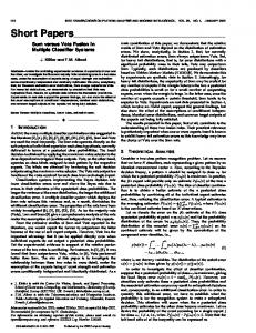
The two methods were tested on four different problems. In the first problem (GSRect), two rectangles are created centered around the origin of a two dimensional space with one rectangle (inner rectangle) accommodating the second (outer rectangle). The size of the initial inner rectangle varies between a side length of 0.1 and 2. The outer rectangle has always twice the side length of the inner rectangle. After the initial cycle, the rectangles undergo three cycles where they grow followed by two cycles where they shrink. After these six-cycles, the rectangles are reset and recentered. This six–cycle behavior is repeated twice to generate a twelve–cycle period. In each cycle a thousand instances are sampled uniformly at random with equal class distributions. The instances that fall inside the inner rectangle are considered positive while those falling in the area of the intersection of the two rectangles are considered negative. Four different growing/shrinking factors are considered: 10%, 25%, 50% and 100%. Each time the model changes, the boundaries of the rectangles are enlarged/reduced by this factor. The growing factor represents a measure of the force on the environment. The larger the growing/shrinking factor, the more severe the change is. Figure 1 shows 6 cycles of this problem using 25% growth factor, three of them growing and three of them shrinking. In the second experiment, we fix the size of the outer rectangle and create a number of inner rectangles. The change occurs by moving the inner rectangles around inside the outer rectangle. We experimented with one and ten inner rectangles. The outside rectangle is a square of length five. In the case of one rectangle, the inner rectangle is a square with sides of length two. After each cycle the inner square is moved between zero and one units in the x and y direction uniformly randomly (random numbers are synchronized to allow a fair comparison between the two systems). In the case of ten rectangles, each rectangle is a square with side lengths one. After each cycle, each square is moved uniformly randomly between zero and 0.25 units in both directions. This experiment tests the ability of the classifier to approximate local and discrete regions. In the first case (Figure 2), a single rectangle is moving around so that boundaries are neither increased nor decreased. In the second case, a representation that identifies ten rectangles (Figure 3) needs to be adapted requiring the maintenance of a moderately high number of rules. The third experiment breaks the axis-parallel convention introducing an oblique dataset. The data are generated according to the rotating tao problem (27) (Figure 4). In this problem, the decision boundary is difficult to approximate using axis–parallel hyper–planes because of its non–linear shape. The experiment examines the effect of oblique decision boundaries on the classifier. Each cycle, the Tao figure is rotated by 30 degrees. In the fourth experiment, we fix the growing/shrinking factor in the first experiment to 25% and add noise to the output. We vary the noise level between 5% and 20% in steps of 5%. For each instance, the class is flipped with a probability equal to the noise level. This experiment tests the impact of noise on the classifier.
5.2
Results
All experiments presented are averaged over one hundred independent runs. The randomnumber generators for the problem generation are synchronized so that GAssist and XCS faced identical hundred problem settings for each problem. The average accuracy and stability for the first three experiments are presented in Tables 1 and 2. The response rate is depicted in
13
Figures 5 to 16 measuring the cumulative performance in the event of a new cycle cumulatively averaging over each 100 steps. The actual online performance is shown in Figures 19 to 30. It is clear that the size of the window plays an important role for GAssist. The larger the window size, the better the average accuracy achieved as shown in Table 1. Stability is not affected significantly. The comparative performances can be found in Figures 5, 6, and 7. It can be seen that a larger window size enables GAssist to reach higher performance. Also, the drop in performance becomes more severe when larger window sizes are used. This drop is most significant after 6000 steps in which the rectangle (after three growing and three shrinking steps) is reset. In the case of a window of size 25 (Figure 5) this drop is not as significant because the learned boundaries are fluctuating due to the small window size so that the approximative bound is actually beneficial in this case. Similar observations can be made in the other dynamic problems. In XCS, the population size has a somewhat similar adaptive influence. Since XCS’s problem representation evolves many smaller rectangles instead of the one rectangle that fits the data best (as GAssist tends to do), a larger population size coincides with a larger memory. Thus, a larger population size enables XCS to reach higher accuracy but the performance drops due to a concept drift are more significant. Especially in the case of ten rectangles (Figure 14), larger population sizes have a strong impact on performance and on the adaptation speed with respect to the problem dynamics. This effect is also reflected in the stability measures shown in Table 2. The larger the population size, the less stable the adaptation due to stronger memory effects that can have positive or negative performance influences. Interestingly, XCS shows a significant performance drop after 6000 steps. The drop is particularly strong when the force of change is set small (compare 10 vs. 50 in Figure 8). Apparently, since XCS’s problem representation converged more to the actual problem, a reset makes adaptation harder for XCS. The convergence can be partially inferred from the population size in the end of a run which is at 353.45 (17.437) in the case of a growing/shrinking factor of 10 but at the larger size 409.24 (18.334) in the case of a growing/shrinking factor of 50. Thus, the less distributed representation slows down adaptation after a concept drift. Comparing XCS directly with GAssist, XCS has a better average accuracy as compared to GAssist with window-25, a comparable one with window-50 and a slightly worse performance with window-100. In this respect, XCS is somehow better in the sense that it does not rely on an appropriate window size. However, population size needs to be chosen sufficiently large. In general, despite the very different problem representations, both system are able to adapt to the different problem settings and dynamics similarly well. It is clear that the larger the change, the more impact it has on the performance of both learning systems. One can argue that both methods are robust in terms of their performance as their average accuracy does not deteriorate much when the change becomes more severe. The decline in average accuracy when comparing growing/shrinking factors of 10% to 100% is less than 0.04 loss of accuracy. This level of robustness is reasonably good when looking at the severity of the change. However, especially the respective cumulative curves show that XCS needs more time to learn the problem initially. Several reasons explain this observation. First, as mentioned above, XCS’s problem representation is much more distributed—especially early in the run—and also depends 14
on the choice of covering size. In our settings, covering generates classifiers that specify rather small hyper-rectangles and thus XCS’s representation starts out with a much more distributed representation than GAssist. Second, GAssist has the additional bit that ignores a problem boundary (partially mimicked by the additional mutation operator µb in XCS). Thus, GAssist is better suited to approximate the initial concept by a random initialization and choice of best current classifier. Finally, XCS learns from each problem instance only once. GAssist on the other hand keeps a window of problem instances form which it learns each iteration. Thus, effectively GAssist learns from each problem instance as often as the size of the window. This clearly gives an advantage to GAssist. Nonetheless, once XCS evolved an approximate problem representation, its adaptive speed and reached accuracy are comparable to the one of GAssist. When comparing XCS and GAssist on the one and ten moving rectangles, GAssist’s performance is better in the former, whereas XCS’s performance is better in the latter. This was expected due to the different problem representations. For GAssist, the maintenance of ten different rules is quite hard whereas XCS naturally maintains a distributed representation. Clearly, when increasing the population size in XCS, performance increases since the different problem niches are less disrupted. Additionally, though, even a window of size 100 is not sufficient to learn the problem with ten rectangles as accurate as XCS does. However, larger window sizes will inevitably delay the adaptation process. Thus, the more complex the concept underlying the problem, the more adaptation speed will need to be traded off by a sufficiently large window.
Table 1: GAssist: Average accuracy and stability in the experiments with different amounts of growing, shrinking, or moving rectangles. The three different window sizes show GAssist’s dependence on a proper problem sample. Problem Window-25 Window-50 Window-100 Type Accuracy Stability Accuracy Stability Accuracy Stability GSRect Gr10 0.9153 0.0054 0.9580 0.0071 0.9706 0.0063 GSRect Gr25 0.9149 0.0049 0.9522 0.0056 0.9623 0.0060 GSRect Gr50 0.9028 0.0069 0.9381 0.0059 0.9503 0.0053 GSRect Gr100 0.8744 0.0136 0.9134 0.0148 0.9260 0.0116 MoveRect 1 0.9425 0.0013 0.9643 0.0015 0.9725 0.0037 MoveRect 10 0.7053 0.0080 0.7680 0.0053 0.8300 0.0096 0.8345 0.0071 0.8606 0.0090 0.8788 0.0054 RotatingTAO
The average accuracy and stability in the experiments with added noise are depicted in Table 3, the response rate is depicted in Figures 17 and 18, and the online performance in Figures 31 and 32 where the performance of both methods is compared varying the noise level in the data. It is clear that a larger window is necessary for GAssist to be effective. In practice, one would learn an appropriate window by using a dynamic window approach as in (26). Comparing window size 100 in GAssist with a population size of 1000 in XCS, performance is very similar. However, XCS seems to approximate the underlying concept slightly more accurately as indicated by the slightly higher average accuracy and in particular by the larger gaps in the event of a concept change (Figure 31 vs. Figure 32).
15
Table 2: GAssist: Average accuracy and stability in the experiments with different amounts of growing, shrinking, or moving rectangles. The three different window sizes show GAssist’s dependence on a proper problem sample. XCS: Average accuracy and stability in the experiments with different amounts of growing, shrinking, or moving rectangles. The increase in the population size in the case of one and ten moving rectangles shows that especially in the case of ten rectangles performance is significantly improved. The Stab-1 measure excludes the first Force level (first 1000 steps) from the determination of the Force since XCS’s initial adaptation speed is slow so that real adaptation comes in only after the representation itself adapted to the underlying problem space. Problem Type GSRect 10 GSRect 25 GSRect 50 GSRect 100 MoveRect 01 MoveRect 10 RotatingTAO
Accuracy 0.9571 0.9517 0.9419 0.9244 0.9302 0.8072 0.8570
N=500 Stability (Stab-1) 0.0355 (0.0241) 0.0241 (0.0136) 0.0167 (0.0084) 0.0158 (0.0125) 0.0187 (0.0071) 0.0176 (0.0057) 0.0149 (0.0151)
Accuracy 0.9619 0.9564 0.9491 0.9353 0.9392 0.8537 0.8643
N=1000 Stability (Stab-1) 0.0335 (0.0233) 0.0244 (0.0128) 0.0166 (0.0077) 0.0180 (0.0118) 0.0210 (0.0087) 0.0268 (0.0092) 0.0145 (0.0133)
Accuracy 0.9634 0.9583 0.9524 0.9426 0.9436 0.8696 0.8664
N=2000 Stability (Stab-1) 0.0316 (0.0206) 0.0246 (0.0121) 0.0186 (0.0081) 0.0189 (0.0116) 0.0192 (0.0079) 0.0345 (0.0132) 0.0149 (0.0127)
Table 3: Average accuracy and stability over all cycles and runs for GAssist with window size of 100 and XCS when adding noise and growing factor of 0.25. Problem Type GSRect Noise5 GSRect Noise10 GSRect Noise15 GSRect Noise20 Problem Type GSRect Noise5 GSRect Noise10 GSRect Noise15 GSRect Noise20
6
N=500 Accuracy Stability (Stab-1) 0.8985 0.0231 (0.0136) 0.8438 0.0244 (0.0136) 0.7863 0.0230 (0.0144) 0.7211 0.0205 (0.0132) Window=25 Accuracy Stability 0.8284 0.0055 0.7575 0.0029 0.6918 0.0041 0.6432 0.0042
XCS N=1000 Accuracy Stability (Stab-1) 0.9030 0.0227 (0.0116) 0.8511 0.0222 (0.0119) 0.7973 0.0238 (0.0122) 0.7398 0.0213 (0.0124) GAssist Window=50 Accuracy Stability 0.8707 0.0037 0.8049 0.0037 0.7476 0.0065 0.6894 0.0072
N=2000 Accuracy Stability (Stab-1) 0.9043 0.0231 (0.0112) 0.8527 0.0235 (0.0116) 0.8012 0.0227 (0.0111) 0.7468 0.0224 (0.0113) Window=100 Accuracy Stability 0.9015 0.0057 0.8426 0.0051 0.7809 0.0053 0.7227 0.0051
Summary and Conclusions
In this paper, we formalized the concept of dynamic environments in the data mining domain and proposed a number of measures to test the performance of different methods. The introduction of a dynamic force showed that data dynamics can and should be quantified. The qualitative classification of different types of dynamics gives additional comparative capabilities. Our focus was on dynamics in which decision boundaries are changed directly (by modifying the target concept). However, other dynamics are interesting to consider in further studies such as the 16
addition of classes or features, noise variations, or sampling bias variations in class distribution or instance space distribution. Our comparative study investigated different dynamic data mining problems in which the model (that is, the concept underlying the data) changed. We compared two genetics-based machine learning systems: GAssist, a Pitt-style approach, and XCS, a Michigan approach. The main findings of the experiments confirm our intuitive understanding of the behavior of both classifiers. On the one hand, GAssist is more suitable for batch learning and approximates decision boundaries globally. The side effects of these two characteristics are: (1) its performance depends on the size of the window; and (2) when the decision regions are isolated discrete areas, it finds it difficult to approximate the decision boundary locally. On the other hand, XCS approximates the decision region through orthogonal sequences of local approximations. This makes it more suitable when the decision regions are locally isolated. However, also XCS’s adaptivity is dependent on parameter settings, such as the investigated population size. As expected by our quantification of force, stronger dynamic forces have a stronger impact on adaptation speed and accuracy. Additionally, the complexity of the underlying concept can have a strong impact on performance and adaptivity. In the case of axis-parallel hyper-rectangles, XCS and GAssist’s problem representation matches the concept space. The more rectangles are added, the more information is needed to learn the problem and thus a larger window is needed. Thus, for future work the definition of problem dynamics might be extended to also quantify problem complexity. Alternatively, since problem complexity is very much dependent on representation, dynamic quantifications, such as the introduced force, need to be kept problem dependent. The quantitative and qualitative insights gained in this paper lead to several paths for future research. First, the current definition of volume is still not general enough to capture any type of dynamics and might be generalized towards a volume of concept space change. The other measure may be adjusted accordingly. On the other hand, the gained understanding of dynamics suggests to feedback this knowledge into the actual learning system. Different types of dynamics should be handled differently by the applied learner. In the case of our evolutionary learning systems, adaptivity can be manipulated by biasing covering operators, mutation and crossover operators, as well as the frequency of GA application. For example, if our system knew that currently the space of positive instances is expected to grow/shrink mutation might cause to expand classifier coverage of positive instances. Additionally, the GA frequency might be increased close to a concept change to introduce more diversity into the population effectively increasing adaptivity. However, additional complexity might need to be added if the learner needs to learn to predict the problem dynamics on its own. With our quantifications of problem dynamics at hand, future work can investigate to what extend knowledge about problem dynamics can improve speed of adaptation and classification accuracy dependent on the type and amount of problem dynamics as well as how difficult it might be to predict different types and amounts of problem dynamics.
7
Acknowledgments
This work was sponsored by the Air Force Office of Scientific Research, Air Force Materiel Command, USAF, under grant F49620-03-1-0129, and by the Technology Research Center (TRECC), a program of the University of Illinois at Urbana-Champaign, administered by the National Center
17
for Supercomputing Applications (NCSA) and funded by the Office of Naval Research under grant N00014-01-1-0175. Research funding for this work was also provided by a grant from the National Science Foundation under grant DMI-9908252. The US Government is authorized to reproduce and distribute reprints for Government purposes notwithstanding any copyright notation thereon. The views and conclusions contained herein are those of the authors and should not be interpreted as necessarily representing the official policies or endorsements, either expressed or implied, of the Air Force Office of Scientific Research, the National Science Foundation, or the U.S. Government. During this work, Hussein Abbass was supported by funding from the following organizations: the Illinois Genetic Algorithm Laboratory, University of New South Wales, and the ARC Centre on Complex Systems grant number CEO0348249. Jaume Bacardit was supported by the Department of Universities, Research and Information Society (DURSI) of the Autonomous Government of Catalonia under grant 2001FI 00514. Martin Butz was supported by the German research foundation (DFG) under grant DFG HO1301/4-3. Additional support from the Computational Science and Engineering graduate option program (CSE) at the University of Illinois at Urbana-Champaign is acknowledged.
18
References [1] H.A. Abbass, “Speeding up back-propagation using multiobjective evolutionary algorithms,” Neural Computation, vol. 15, no. 11, pp. 2705–2726, 2003. [2] J.H. Holland, Adaptation in natural and artificial systems, MIT press, second edition, 1998. [3] J.H. Holland, L.B. Booker, M. Colombetti, M. Dorigo, D.E. Goldberg, S. Forrest, R.L. Riolo, R.E. Smith, P.L. Lanzi, W. Stolzmann, and S.W. Wilson, “What is a Learning Classifier System?,” in Learning Classifier Systems. From Foundations to Applications, Pier Luca Lanzi, Wolfgang Stolzmann, and Stewart W. Wilson, Eds., Berlin, 2000, vol. 1813 of LNAI, pp. 3–32, Springer-Verlag. [4] L.B. Booker, Intelligent Behavior as an Adaptation to the Task Environment, Ph.D. thesis, The University of Michigan, 1982. [5] Rick L. Riolo, “Bucket Brigade Performance: I. Long Sequences of Classifiers,” in Proceedings of the 2nd International Conference on Genetic Algorithms (ICGA87), John J. Grefenstette, Ed., Cambridge, MA, July 1987, pp. 184–195, Lawrence Erlbaum Associates. [6] Stewart W. Wilson, “Classifier fitness based on accuracy,” Evolutionary Computation, vol. 3, no. 2, pp. 149–175, 1995. [7] K.A. De Jong, “Learning with Genetic Algorithms: An Overview,” Machine Learning, vol. 3, pp. 121–138, 1988. [8] P. Collard, C. Escazut, and E. Gaspar, “An evolutionnary approach for time dependant optimization,” International Journal on Artificial Intelligence Tools, pp. 665–695, 1997. [9] M. Kirley, “An empirical investigation of optimisation in dynamic environments using the cellular genetic algorithm,” in Genetic and Evolutionary Computation Conference, 2000, pp. 1–18. [10] D.E. Goldberg, Genetic algorithms: in search, optimisation and machine learning, Addison Wesely, 1989. [11] J. Branke, Evolutionary Optimization in Dynamic Environments, Kluwer Academic Publishers, Boston, 2001. [12] D. Mladenic, “Machine learning used by personal webwatcher,” in Proceedings of ACAI-99 Workshop on Machine Learning and Intelligent Agents, 1999. [13] V. Petridis and Ath. Kehagias, “Modular neural networks for map classification of time series and the partition algorithm,” IEEE Trans. on Neural Networks, vol. 7, pp. 73–86, 1996. [14] B. Horne and C. Giles, “An experimental comparison of recurrent neural networks,” in Advances in neural information processing systems (NIPS), G. Tesauro, D. Touretzky, and T. Leen, Eds. 1995, vol. 7, pp. 697–704, MIT Press. [15] W. Lin, M.A. Orgun, and G.J. Williams, “Multilevels hidden markov models for temporal data mining,” in Proceedings of the 2001 KDD Workshop on Temporal Data Mining, 2001. [16] R.D. Martin and V. Yohai, “Data mining for unusual movements in temporal data,” in Proceedings of the 2001 KDD Workshop on Temporal Data Mining, 2001.
19
[17] M. Kubat and G. Widmer, “Adapting to drift in continuous domains,” in Lecture Notes in Computer Science, 1995, vol. 912, pp. 307–310. [18] P.E. Utgoff, “Incremental induction of decision trees,” Machine Learning, vol. 4, pp. 161–186, 1989. [19] M.B. Harries, C. Sammut, and K. Horn, “Extracting hidden context,” Machine Learning, vol. 32, pp. 101–126, 1998. [20] E. Keogh and S. Kasetty, “On the need for time series data mining benchmarks: a survey and empirical demonstration,” in SIGKDD ’02, 2002. [21] Jaume Bacardit and Josep M. Garrell, “Evolving multiple discretizations with adaptive intervals for a pittsburgh rule-based learning classifier system,” in Proceedings of the Genetic and Evolutionary Computation Conference - GECCO2003. 2003, pp. 1818–1831, LNCS 2724, Springer. [22] Kenneth A. DeJong, William M. Spears, and Diana F. Gordon, “Using genetic algorithms for concept learning,” Machine Learning, vol. 13, no. 2/3, pp. 161–188, 1993. [23] J. Rissanen, “Modeling by shortest data description,” Automatica, vol. vol. 14, pp. 465–471, 1978. [24] Jaume Bacardit and Josep M. Garrell, “Bloat control and generalization pressure using the minimum description length principle for a pittsburgh approach learning classifier system,” in Proceedings of the 6th International Workshop on Learning Classifier Systems. 2003, (in press), LNAI, Springer. [25] Stewart W. Wilson, “Get real! XCS with continuous-valued inputs,” in Festschrift in Honor of John H. Holland, L. Booker, Stephanie Forrest, M. Mitchell, and Rick L. Riolo, Eds. 1999, pp. 111–121, Center for the Study of Complex Systems. [26] Gerhard Widmer and Miroslav Kubat, “Learning flexible concepts from streams of examples: FLORA 2,” in European Conference on Artificial Intelligence, 1992, pp. 463–467. [27] Xavier Llor`a and Josep M. Garrell, “Evolving Partially-Defined instances with Evolutionary Algorithms,” in Proceedings of the 18th International Conference on Machine Learning (ICML’2001). 2001, pp. 337–344, Morgan Kauffmann.
20
Cycle 1
Cycle 2
1.5
Cycle 3
1.5
1.5
Class 0 Class 1
Class 0 Class 1
Class 0 Class 1
1
1
1
0.5
0.5
0.5
0
0
0
-0.5
-0.5
-0.5
-1
-1
-1
-1.5
-1.5
-1.5
-2
-1
0
1
2
-2
-1
Cycle 4
0
1
2
-2
1.5
1.5
Class 0 Class 1 1
0.5
0.5
0.5
0
0
0
-0.5
-0.5
-0.5
-1
-1
-1
-1.5 0
1
2
Class 0 Class 1 1
-1
1
1.5
Class 0 Class 1
-1.5
0 Cycle 6
1
-2
-1
Cycle 5
-1.5
2
-2
-1
0
1
2
-2
-1
0
1
2
Figure 1: GSRect dynamic dataset with 3 growing and 3 shrinking cycles and 25% growth factor Cycle 1
Cycle 2 Class 0 Class 1
2
Cycle 3 Class 0 Class 1
2
1
1
1
0
0
0
-1
-1
-1
-2
-2 -2
-1
0
1
2
Class 0 Class 1
2
-2 -2
-1
0
1
2
-2
-1
Figure 2: 3 cycles of the moving 1 rectangle dataset
21
0
1
2
Cycle 1
Cycle 2 Class 0 Class 1
2
Cycle 3 Class 0 Class 1
2
1
1
1
0
0
0
-1
-1
-1
-2
-2 -2
-1
0
1
Class 0 Class 1
2
-2
2
-2
-1
0
1
2
-2
-1
0
1
2
Figure 3: 3 cycles of the moving 10 rectangles dataset
Cycle 1
Cycle 2
6
Cycle 3
6
6
Class 0 Class 1
Class 0 Class 1
Class 0 Class 1
4
4
4
2
2
2
0
0
0
-2
-2
-2
-4
-4
-4
-6
-6 -6
-4
-2
0
2
4
6
-6 -6
-4
-2
0
2
4
6
-6
-4
Figure 4: 3 cycles of the rotating TAO dataset
22
-2
0
2
4
6
0.8
0.8
0.7
0.7
0.6
0.5
0.4
0.6
0.5
0.4
0.3
0.3
0.2
0.2
0.1
0.1
0
Accumulated Average
Accumulated Average
1
0.9
0
2000
4000
6000 Time
8000
10000
0
12000
1
1
0.9
0.9
0.8
0.8
0.7
0.7 Accumulated Average
Accumulated Average
1
0.9
0.6
0.5
0.4
0.2
0.1
0.1
4000
6000 Time
8000
10000
12000
6000 Time
8000
10000
12000
0
2000
4000
6000 Time
8000
10000
12000
0.4
0.3
2000
4000
0.5
0.2
0
2000
0.6
0.3
0
0
0
Figure 5: The cumulative average performance using GAssist for the GSRect problem with window 25 and growth factors of 10, 25, 50, 75, and 100 ordered from left to right top down respectively.
23
0.8
0.8
0.7
0.7
0.6
0.5
0.4
0.6
0.5
0.4
0.3
0.3
0.2
0.2
0.1
0.1
0
Accumulated Average
Accumulated Average
1
0.9
0
2000
4000
6000 Time
8000
10000
0
12000
1
1
0.9
0.9
0.8
0.8
0.7
0.7 Accumulated Average
Accumulated Average
1
0.9
0.6
0.5
0.4
0.2
0.1
0.1
4000
6000 Time
8000
10000
12000
6000 Time
8000
10000
12000
0
2000
4000
6000 Time
8000
10000
12000
0.4
0.2
2000
4000
0.5
0.3
0
2000
0.6
0.3
0
0
0
Figure 6: The cumulative average performance using GAssist for the GSRect problem with window 50 and growth factors of 10, 25, 50, and 100 ordered from left to right top down respectively.
24
0.8
0.8
0.7
0.7
0.6
0.5
0.4
0.6
0.5
0.4
0.3
0.3
0.2
0.2
0.1
0.1
0
Accumulated Average
Accumulated Average
1
0.9
0
2000
4000
6000 Time
8000
10000
0
12000
1
1
0.9
0.9
0.8
0.8
0.7
0.7 Accumulated Average
Accumulated Average
1
0.9
0.6
0.5
0.4
0.2
0.1
0.1
4000
6000 Time
8000
10000
12000
6000 Time
8000
10000
12000
0
2000
4000
6000 Time
8000
10000
12000
0.4
0.2
2000
4000
0.5
0.3
0
2000
0.6
0.3
0
0
0
Figure 7: The cumulative average performance using GAssist for the GSRect problem with window 100 and growth factors of 10, 25, 50, and 100 ordered from left to right top down respectively.
25
1
0.8
0.8
0.6
0.6 Performance
Performance
1
0.4
0.2
0.4
0.2
0
0 0
2000
4000
6000
8000
10000
12000
0
2000
4000
6000
8000
10000
12000
8000
10000
12000
Time
1
1
0.8
0.8
0.6
0.6 Performance
Performance
Time
0.4
0.2
0.4
0.2
0
0 0
2000
4000
6000
8000
10000
12000
Time
0
2000
4000
6000 Time
Figure 8: The cumulative average performance using XCS with population size N=500 for the GSRect problem with growing/shrinking factors of 10, 25, 50, and 100 ordered from left to right top down respectively.
26
1
0.8
0.8
0.6
0.6 Performance
Performance
1
0.4
0.2
0.4
0.2
0
0 0
2000
4000
6000
8000
10000
12000
0
2000
4000
6000
8000
10000
12000
8000
10000
12000
Time
1
1
0.8
0.8
0.6
0.6 Performance
Performance
Time
0.4
0.2
0.4
0.2
0
0 0
2000
4000
6000
8000
10000
12000
Time
0
2000
4000
6000 Time
Figure 9: The cumulative average performance using XCS with population size N=1000 for the GSRect problem with growing/shrinking factors of 10, 25, 50, and 100 ordered from left to right top down respectively.
27
1
0.8
0.8
0.6
0.6 Performance
Performance
1
0.4
0.2
0.4
0.2
0
0 0
2000
4000
6000
8000
10000
12000
0
2000
4000
6000
8000
10000
12000
8000
10000
12000
Time
1
1
0.8
0.8
0.6
0.6 Performance
Performance
Time
0.4
0.2
0.4
0.2
0
0 0
2000
4000
6000
8000
10000
12000
0
2000
4000
6000
Time
Time
1
1
0.9
0.9
0.8
0.8
0.8
0.7
0.7
0.7
0.6
0.5
0.4
Accumulated Average
1
0.9
Accumulated Average
Accumulated Average
Figure 10: The cumulative average performance using XCS with population size N=2000 for the GSRect problem with growing/shrinking factors of 10, 25, 50, and 100 ordered from left to right top down respectively.
0.6
0.5
0.4
0.6
0.5
0.4
0.3
0.3
0.3
0.2
0.2
0.2
0.1
0.1
0
0
1000
2000
3000
4000
5000 Time
6000
7000
8000
9000
10000
0
0.1
0
1000
2000
3000
4000
5000 Time
6000
7000
8000
9000
10000
0
0
1000
2000
3000
4000
5000 Time
6000
7000
8000
9000
10000
Figure 11: The cumulative average performance using GAssist for the MoveRect problem with 1 rectangle with window size of 25 (left most column); 50 (middle column); and 100 (right column).
28
1
0.8
0.8
0.8
0.6
0.6
0.6
0.4
Performance
1
Performance
Performance
1
0.4
0.2
0.2
0
0.2
0 0
2000
4000
6000
8000
10000
12000
0.4
0 0
2000
4000
Time
6000
8000
10000
12000
0
2000
4000
6000
Time
8000
10000
12000
Time
1
1
0.9
0.9
0.8
0.8
0.8
0.7
0.7
0.7
0.6
0.5
0.4
Accumulated Average
1
0.9
Accumulated Average
Accumulated Average
Figure 12: The cumulative average performance using XCS on the MoveRect problem with one rectangle and population sizes of 500, 1000, and 2000 ordered from left to right, respectively.
0.6
0.5
0.4
0.6
0.5
0.4
0.3
0.3
0.3
0.2
0.2
0.2
0.1
0.1
0
0
1000
2000
3000
4000
5000 Time
6000
7000
8000
9000
0
10000
0.1
0
1000
2000
3000
4000
5000 Time
6000
7000
8000
9000
10000
0
0
1000
2000
3000
4000
5000 Time
6000
7000
8000
9000
10000
1
1
0.8
0.8
0.8
0.6
0.6
0.6
0.4
0.2
Performance
1
Performance
Performance
Figure 13: The cumulative average performance using GAssist for the MoveRect problem with 10 rectangles with window size of 25 (left most column); 50 (middle column); and 100 (right column).
0.4
0.2
0
0.2
0 0
2000
4000
6000 Time
8000
10000
12000
0.4
0 0
2000
4000
6000 Time
8000
10000
12000
0
2000
4000
6000
8000
10000
12000
Time
Figure 14: The cumulative average performance using XCS on the MoveRect problem with 10 rectangles and population sizes of 500, 1000, and 2000 ordered from left to right, respectively.
29
1
0.9
0.8
0.8
0.8
0.7
0.7
0.7
0.6
0.5
0.4
Accumulated Average
1
0.9
Accumulated Average
Accumulated Average
1
0.9
0.6
0.5
0.4
0.6
0.5
0.4
0.3
0.3
0.3
0.2
0.2
0.2
0.1
0.1
0
0
1000
2000
3000
4000
5000 Time
6000
7000
8000
9000
0
10000
0.1
0
1000
2000
3000
4000
5000 Time
6000
7000
8000
9000
10000
0
0
1000
2000
3000
4000
5000 Time
6000
7000
8000
9000
10000
1
1
0.8
0.8
0.8
0.6
0.6
0.6
0.4
0.2
Performance
1
Performance
Performance
Figure 15: The cumulative average performance using GAssist for the RotatingTAO problem with window size of 25 (left most column); 50 (middle column); and 100 (right column).
0.4
0.2
0
0.2
0 0
2000
4000
6000 Time
8000
10000
12000
0.4
0 0
2000
4000
6000 Time
8000
10000
12000
0
2000
4000
6000
8000
10000
12000
Time
Figure 16: The cumulative average performance using XCS on the RotatingTAO problem with population sizes of 500, 1000, and 2000 ordered from left to right, respectively.
30
0.8
0.8
0.7
0.7
0.6
0.5
0.4
0.6
0.5
0.4
0.3
0.3
0.2
0.2
0.1
0.1
0
Accumulated Average
Accumulated Average
1
0.9
0
2000
4000
6000 Time
8000
10000
0
12000
1
1
0.9
0.9
0.8
0.8
0.7
0.7 Accumulated Average
Accumulated Average
1
0.9
0.6
0.5
0.4
0.2
0.1
0.1
4000
6000 Time
8000
10000
12000
6000 Time
8000
10000
12000
0
2000
4000
6000 Time
8000
10000
12000
0.4
0.2
2000
4000
0.5
0.3
0
2000
0.6
0.3
0
0
0
Figure 17: The cumulative average performance using GAssist with window size 100 for the GSRect problem with noise levels of 5%, 10%, 15%, and 20% from left to right top down respectively.
31
1
0.8
0.8
0.6
0.6 Performance
Performance
1
0.4
0.2
0.4
0.2
0
0 0
2000
4000
6000
8000
10000
12000
0
2000
4000
6000
8000
10000
12000
8000
10000
12000
Time
1
1
0.8
0.8
0.6
0.6 Performance
Performance
Time
0.4
0.2
0.4
0.2
0
0 0
2000
4000
6000
8000
10000
12000
Time
0
2000
4000
6000 Time
Figure 18: The cumulative average performance using XCS with population size N=1000 for the GSRect problem with noise levels of 5%, 10%, 15%, and 20% from left to right top down respectively.
32
1
0.8
0.8
0.6
0.6 Performance
Performance
1
0.4
0.2
0.4
0.2
0
0 0
2000
4000
6000
8000
10000
12000
0
2000
4000
6000
8000
10000
12000
8000
10000
12000
Time
1
1
0.8
0.8
0.6
0.6 Performance
Performance
Time
0.4
0.2
0.4
0.2
0
0 0
2000
4000
6000
8000
10000
12000
Time
0
2000
4000
6000 Time
Figure 19: The online performance for the GAssist on the GSRect problem using window size of 25 and growing/shrinking factors of 10, 25, 50, and 100 ordered from left to right top down respectively.
33
1
0.8
0.8
0.6
0.6 Performance
Performance
1
0.4
0.2
0.4
0.2
0
0 0
2000
4000
6000
8000
10000
12000
0
2000
4000
6000
8000
10000
12000
8000
10000
12000
Time
1
1
0.8
0.8
0.6
0.6 Performance
Performance
Time
0.4
0.2
0.4
0.2
0
0 0
2000
4000
6000
8000
10000
12000
Time
0
2000
4000
6000 Time
Figure 20: The online performance for the GAssist on the GSRect problem using window size of 50 and growing/shrinking factors of 10, 25, 50, and 100 ordered from left to right top down respectively.
34
1
0.8
0.8
0.6
0.6 Performance
Performance
1
0.4
0.2
0.4
0.2
0
0 0
2000
4000
6000
8000
10000
12000
0
2000
4000
6000
8000
10000
12000
8000
10000
12000
Time
1
1
0.8
0.8
0.6
0.6 Performance
Performance
Time
0.4
0.2
0.4
0.2
0
0 0
2000
4000
6000
8000
10000
12000
Time
0
2000
4000
6000 Time
Figure 21: The online performance for the GAssist on the GSRect problem using window size of 100 and growing/shrinking factors of 10, 25, 50, and 100 ordered from left to right top down respectively.
35
1
0.8
0.8
0.6
0.6 Performance
Performance
1
0.4
0.2
0.4
0.2
0
0 0
2000
4000
6000
8000
10000
12000
0
2000
4000
6000
8000
10000
12000
8000
10000
12000
Time
1
1
0.8
0.8
0.6
0.6 Performance
Performance
Time
0.4
0.2
0.4
0.2
0
0 0
2000
4000
6000
8000
10000
12000
Time
0
2000
4000
6000 Time
Figure 22: The online performance for the XCS with population size N=500 on the GSRect problem using growing/shrinking factors of 10, 25, 50, and 100 ordered from left to right top down respectively.
36
1
0.8
0.8
0.6
0.6 Performance
Performance
1
0.4
0.2
0.4
0.2
0
0 0
2000
4000
6000
8000
10000
12000
0
2000
4000
6000
8000
10000
12000
8000
10000
12000
Time
1
1
0.8
0.8
0.6
0.6 Performance
Performance
Time
0.4
0.2
0.4
0.2
0
0 0
2000
4000
6000
8000
10000
12000
Time
0
2000
4000
6000 Time
Figure 23: The online performance for the XCS with population size N=1000 on the GSRect problem using growing/shrinking factors of 10, 25, 50, and 100 ordered from left to right top down respectively.
37
1
0.8
0.8
0.6
0.6 Performance
Performance
1
0.4
0.2
0.4
0.2
0
0 0
2000
4000
6000
8000
10000
12000
0
2000
4000
6000
8000
10000
12000
8000
10000
12000
Time
1
1
0.8
0.8
0.6
0.6 Performance
Performance
Time
0.4
0.2
0.4
0.2
0
0 0
2000
4000
6000
8000
10000
12000
Time
0
2000
4000
6000 Time
Figure 24: The online performance for the XCS with population size N=2000 on the GSRect problem using growing/shrinking factors of 10, 25, 50, and 100 ordered from left to right top down respectively.
38
1
0.8
0.8
0.8
0.6
0.6
0.6
0.4
0.2
Performance
1
Performance
Performance
1
0.4
0.2
0
0.2
0 0
2000
4000
6000
8000
10000
0.4
0 0
2000
4000
Time
6000
8000
10000
0
2000
4000
Time
6000
8000
10000
Time
1
1
0.8
0.8
0.8
0.6
0.6
0.6
0.4
0.2
Performance
1
Performance
Performance
Figure 25: The online performance for the GAsssist on the MoveRect problem with 1 rectangle and window size of 25, 50, and 100 ordered from left to right top down respectively.
0.4
0.2
0
0.2
0 0
2000
4000
6000
8000
10000
12000
0.4
0 0
2000
4000
6000
Time
8000
10000
12000
0
2000
4000
6000
Time
8000
10000
12000
Time
1
1
0.8
0.8
0.8
0.6
0.6
0.6
0.4
0.2
Performance
1
Performance
Performance
Figure 26: The online performance for the XCS on the MoveRect problem with 1 rectangle and population size of 500, 1000, and 2000 ordered from left to right respectively.
0.4
0.2
0
0.2
0 0
2000
4000
6000 Time
8000
10000
0.4
0 0
2000
4000
6000 Time
8000
10000
0
2000
4000
6000
8000
10000
Time
Figure 27: The online performance for the GAsssist on the MoveRect problem with 10 rectangles and window size of 25, 50, and 100 ordered from left to right respectively.
39
1
0.8
0.8
0.8
0.6
0.6
0.6
0.4
0.2
Performance
1
Performance
Performance
1
0.4
0.2
0
0.2
0 0
2000
4000
6000
8000
10000
12000
0.4
0 0
2000
4000
6000
Time
8000
10000
12000
0
2000
4000
6000
Time
8000
10000
12000
Time
1
1
0.8
0.8
0.8
0.6
0.6
0.6
0.4
0.2
Performance
1
Performance
Performance
Figure 28: The online performance for the XCS on the MoveRect problem with 10 rectangles and population size of 500, 1000, and 2000 ordered from left to right respectively.
0.4
0.2
0
0.2
0 0
2000
4000
6000
8000
10000
0.4
0 0
2000
4000
Time
6000
8000
10000
0
2000
4000
Time
6000
8000
10000
Time
1
1
0.8
0.8
0.8
0.6
0.6
0.6
0.4
0.2
Performance
1
Performance
Performance
Figure 29: The online performance for the GAssist on the RotatingTao problem with window size of 25, 50, and 100 ordered from left to right.
0.4
0.2
0
0.2
0 0
2000
4000
6000 Time
8000
10000
12000
0.4
0 0
2000
4000
6000 Time
8000
10000
12000
0
2000
4000
6000
8000
10000
12000
Time
Figure 30: The online performance for the XCS on the RotatingTao problem and population size 500, 1000, and 2000 ordered from left to right respectively.
40
1
0.8
0.8
0.6
0.6 Performance
Performance
1
0.4
0.2
0.4
0.2
0
0 0
2000
4000
6000
8000
10000
12000
0
2000
4000
6000
8000
10000
12000
8000
10000
12000
Time
1
1
0.8
0.8
0.6
0.6 Performance
Performance
Time
0.4
0.2
0.4
0.2
0
0 0
2000
4000
6000
8000
10000
12000
Time
0
2000
4000
6000 Time
Figure 31: The online performance for the GAssist on the GSRect problem with noise using window size of 100 and noise level 5%, 10%, 15%, and 20% ordered from left to right respectively.
41
1
0.8
0.8
0.6
0.6 Performance
Performance
1
0.4
0.2
0.4
0.2
0
0 0
2000
4000
6000
8000
10000
12000
0
2000
4000
6000
8000
10000
12000
8000
10000
12000
Time
1
1
0.8
0.8
0.6
0.6 Performance
Performance
Time
0.4
0.2
0.4
0.2
0
0 0
2000
4000
6000
8000
10000
12000
Time
0
2000
4000
6000 Time
Figure 32: The online performance for the XCS with population size N=1000 on the GSRect problem with noise using noise level 5%, 10%, 15%, and 20% ordered from left to right top down respectively.
42