Online algorithms for partially ordered sets - Helda

Date of acceptance

Instructor

Online algorithms for partially ordered sets Mikko Herranen

Helsinki October 13, 2013 MSc thesis UNIVERSITY OF HELSINKI Department of Computer Science

Grade

HELSINGIN YLIOPISTO — HELSINGFORS UNIVERSITET — UNIVERSITY OF HELSINKI Laitos — Institution — Department

Tiedekunta — Fakultet — Faculty

Faculty of Science

Department of Computer Science

Tekijä — Författare — Author

Mikko Herranen Työn nimi — Arbetets titel — Title

Online algorithms for partially ordered sets Oppiaine — Läroämne — Subject

Computer Science Työn laji — Arbetets art — Level

Aika — Datum — Month and year

Sivumäärä — Sidoantal — Number of pages

MSc thesis

October 13, 2013

50 pages + 1 appendices

Tiivistelmä — Referat — Abstract

Partially ordered sets (posets) have various applications in computer science ranging from database systems to distributed computing. Content-based routing in publish/subscribe systems is a major poset use case. Content-based routing requires efficient poset online algorithms, including efficient insertion and deletion algorithms. We study the query and total complexities of online operations on posets and poset-like data structures. The main data structures considered are the incidence matrix, Siena poset, ChainMerge, and poset-derived forest. The contributions of this thesis are twofold: First, we present an online adaptation of the ChainMerge data structure as well as several novel poset-derived forest variants. We study the effectiveness of a first-fit-equivalent ChainMerge online insertion algorithm and show that it performs close to optimal query-wise while requiring less CPU processing in a benchmark setting. Second, we present the results of an empirical performance evaluation. In the evaluation we compare the data structures in terms of query complexity and total complexity. The results indicate ChainMerge as the best structure overall. The incidence matrix, although simple, excels in some benchmarks. Poset-derived forest is very fast overall if a “true” poset data structure is not a requirement. Placing elements in smaller poset-derived forests and then merging them is an efficient way to construct poset-derived forests. Lazy evaluation for poset-derived forests shows some promise as well. ACM Computing Classification System (CCS): A.1 [Introductory and Survey], E.1 [Data Structures]

Avainsanat — Nyckelord — Keywords

poset, publish-subscribe, benchmark Säilytyspaikka — Förvaringsställe — Where deposited

Muita tietoja — övriga uppgifter — Additional information

ii

Contents 1 Introduction

1

2 Definitions

2

3 Use cases for posets

3

3.1

Publish/subscribe systems . . . . . . . . . . . . . . . . . . . . . . . .

3

3.2

Recommender systems . . . . . . . . . . . . . . . . . . . . . . . . . .

5

4 Problem description

6

4.1

The set of operations . . . . . . . . . . . . . . . . . . . . . . . . . . .

6

4.2

Types of complexities . . . . . . . . . . . . . . . . . . . . . . . . . . .

7

4.3

Certain theoretical lower bounds . . . . . . . . . . . . . . . . . . . . .

8

5 Poset data structures

8

5.1

Incidence matrix . . . . . . . . . . . . . . . . . . . . . . . . . . . . .

8

5.2

Siena filters poset . . . . . . . . . . . . . . . . . . . . . . . . . . . . . 11

5.3

ChainMerge . . . . . . . . . . . . . . . . . . . . . . . . . . . . . . . . 12 5.3.1

Offline insertion algorithms . . . . . . . . . . . . . . . . . . . 13

5.3.2

Online insertion algorithm . . . . . . . . . . . . . . . . . . . . 13

5.3.3

Delete and look-up algorithms . . . . . . . . . . . . . . . . . . 15

5.3.4

Root set computation . . . . . . . . . . . . . . . . . . . . . . . 16

5.3.5

Maintaining a minimum chain decomposition

5.3.6

The Merge algorithm . . . . . . . . . . . . . . . . . . . . . . . 18

. . . . . . . . . 17

5.4

Worst-case complexities . . . . . . . . . . . . . . . . . . . . . . . . . 21

5.5

Other data structures . . . . . . . . . . . . . . . . . . . . . . . . . . . 22

6 Poset-derived forest

22

6.1

Definitions . . . . . . . . . . . . . . . . . . . . . . . . . . . . . . . . . 23

6.2

The algorithms . . . . . . . . . . . . . . . . . . . . . . . . . . . . . . 23

iii 6.3

Balanced PF . . . . . . . . . . . . . . . . . . . . . . . . . . . . . . . . 25

6.4

Lazy-evaluated PF . . . . . . . . . . . . . . . . . . . . . . . . . . . . 26

6.5

PF merging . . . . . . . . . . . . . . . . . . . . . . . . . . . . . . . . 27

7 Experimental evaluation

28

7.1

Input values . . . . . . . . . . . . . . . . . . . . . . . . . . . . . . . . 28

7.2

Element comparison scheme . . . . . . . . . . . . . . . . . . . . . . . 33

7.3

Benchmarking setup . . . . . . . . . . . . . . . . . . . . . . . . . . . 34

7.4

Poset structures: results and analysis . . . . . . . . . . . . . . . . . . 35

7.5

Poset-derived forest: results and analysis . . . . . . . . . . . . . . . . 36

8 Discussion

45

9 Future work

47

10 Conclusions

48

References

48

Appendices 1 Algorithm pseudo code listings

1

1

Introduction

Partially ordered sets or posets have various applications in computer science ranging from database systems to distributed computing. Posets have uses in ranking scenarios where certain pairs of elements are incomparable, such as ranking conference submissions [DKM+ 11]. In a recommender system, a poset data structure may be used to record the partially known preferences of the users [RV97]. In publish/subscribe systems, posets are used for message filtering [TK06] [CRW01]. In database systems, posets can be used e.g. to aid decomposition of a database schema [Heg94]. In this thesis we focus on poset online operations. An online algorithm operates on incomplete information. For example, a content-based router might store the client subscriptions in a poset data structure. The data structure has to be updated every time the clients make changes to their subscriptions; the entire set of input elements cannot be known in advance, which places additional requirements on the poset data structures and algorithms. In contrast, an offline algorithm knows the entire input set in advance and can thus make an optimal choice at each step. With online operations we sometimes have to settle for a non-optimal solution. A poset data structure may have to store large amounts of data. Additionally, the element comparisons might be expensive. This creates a need for efficient poset data structures and algorithms. The online requirement and the use cases considered in this thesis necessitate also fast insertion and deletion operations. We study the complexity of poset online operations on various poset and posetlike data structures. We seek to find the most efficient poset data structures and algorithms in terms of a fixed set of online operations which was chosen to support the online case while remaining small enough to fit in the scope of a master’s thesis. We discuss the issue both from a theoretical and empirical aspect although the focus is on the empirical part. In the empirical part, we present the results of an empirical evaluation that was carried out by implementing all studied data structures from scratch in Java and executing a series of benchmark runs in a controlled environment. This thesis is organized as follows. First, in Section 2 we define the terms and syntax used in the rest of the paper. In Section 3 we study a couple of the poset use cases in more detail. In Section 4 we discuss a few necessary preliminaries before introducing the poset data structures in Section 5 and poset-derived forest in Section 6. In Section 7 we present the results of the experimental evaluation and finally in

2 sections 8 to 10 we discuss the results and possible future work. Algorithm pseudo code listings can be found in the appendix.

2

Definitions

A partially ordered set or poset P is a partial ordering of the elements of a set. Poset P is formally defined as P = (P, ) where P is the set of elements in P and is an irreflexive, transitive binary relation. a b claims element a ∈ P precedes, or dominates, element b ∈ P and a b claims a does not precede b. If either a b or b a holds, the elements are said to be comparable, written as a ∼ b. Otherwise the elements are said to be incomparable, written as a b. An oracle is a theoretical black box that answers queries about the relations of elements. Given elements a and b, the oracle answers with a b, b a, or a b. A chain of P is a subset of mutually comparable elements of P. A chain C ⊆ P is defined as ci , cj ∈ C, i 6= j such that for any ci , cj either ci cj or cj ci holds. An antichain of P is a subset of mutually incomparable elements of P. An antichain A ⊆ P is defined as ai , aj ∈ A, i 6= j such that ai aj for any ai , aj . A chain decomposition of P is a set of chains C ⊆ P such that their union equals P . A minimum chain decomposition of P is a chain decomposition that contains the fewest number of chains possible given P and a maximum chain decomposition of P is a chain decomposition that contains the largest number of chains given P. The width of a poset, w(P), is the number of elements in the largest antichain of the poset [DKM+ 11] [BKS10], which equals the number of chains in a minimum chain decomposition of that poset [Dil50]. For our purposes we also define another width, wmax (P), as the number of chains in a maximum chain decomposition of P. The widths are characterized by the following equation: w(P) ≤ wmax (P) ≤ n, where n is the number of elements in P. The root set of poset P is the set of elements p ∈ P such that pi p for all pi ∈ P, pi 6= p, that is the set of elements that are not covered by any other elements of P. It is also called the non-covered set. The covered set of an element e is a set of elements p ∈ P such that e p.

3

3

Use cases for posets

In this section we briefly discuss two poset use cases in order to provide background for the rest of the paper. In Section 3.1 we discuss content-based routing in the context of publish/subscribe systems, and in Section 3.2 we discuss recommender systems. The treatment given in this section is necessarily brief and the reader is encouraged to read the referenced papers for more information.

3.1

Publish/subscribe systems

A publish/subscribe system decouples the information producers and the information consumers. A publish/subscribe system consists of a set of producers, who publish notifications, a set of consumers, who subscribe to notifications, and a set of message brokers who deliver the notifications from the producers to the subscribers. There are many benefits to publish/subscribe systems. The following benefits are given by Mühl [Müh02]. The first benefit is loose coupling or decoupling in space: the producers need not address or know the consumers and vice versa. According to Mühl, loose coupling “facilitates flexibility and extensibility because new consumers and producers can be added, moved, or removed easily.” [Müh02] The second benefit is asynchronous communication. The third benefit is decoupling in time: the producers and the consumers need not be available at the same time. Publish/subscribe systems can be divided into two broad categories: subject-based systems and content-based systems [LP+ 03]. In a subject-based system each notification belongs under a topic and the consumers subscribe to topics of interest. This has several downsides. First of all, the producer needs to maintain the category of topics and classify each notification. Also, to remain meaningful, the topics must be broad enough, but broader topics make it necessary for the consumers to perform client-side filtering; if the consumer is interested in a narrow subset of the notifications, for example Delta Airlines flights outbound from Miami at certain times, a topic fulfilling those exact criteria most likely does not exist and the consumer must therefore subscribe to one or more broader topics and filter the relevant notifications from all notifications classified under those topics. Content-based systems on the other hand provide the consumer only the information she needs without the need to learn the set of topic names and their content before subscribing [LP+ 03]. In a content-based system the consumers subscribe to notifications by specifying filters in a subscription language [EFGK03]. The filters

4 can contain the basic comparison operators and can be logically combined to produce more complex filters. The filters are then applied to the metadata of each notification to determine whether it matches the filter. For example, a filter such as “airline = delta” would match all notifications of flights operated by Delta Airlines in a hypothetical flight monitoring system. “airline = delta ∧ airport = mia” would match all flights operated by Delta Airlines and flown out of Miami. In a content-based systems the number of unique subscriptions can be considerably larger than in a topic-based system which necessitates efficient matching of notifications to subscriptions [LP+ 03]. The simplest way to implement a distributed notification service is flooding [Müh02]. In the flooding approach a router forwards a notification published by one of its local clients to all neighboring routers. If a router receives a notification from a neighboring router, it simply forwards it to all other neighboring routers. Received notifications are also forwarded to local clients with matching subscriptions. Major drawback of the flooding approach is that a potentially large number of unnecessary notifications are sent since each notification is eventually received by every router in the system regardless of whether there are interested parties to whom it can forward the notification. The opposite approach to flooding is content-based routing. In content-based routing the notifications are routed based on their contents. Specifically, a notification is sent to a router only if it can forward the notification to an interested party (a client or another router). Covering-based routing is a special case of content-based routing. In covering-based routing the covering relation of filters is exploited [Müh02]. A filter f1 is said to cover another filter f2 if f1 matches all notifications f2 matches. The covering relations of a set of filters impose a partial order on the set. Systems such as Siena exploit the covering-based partial order by storing the client subscriptions in a poset data structure. The following example is based on the description of Siena by the Siena authors [CRW01]. Figure 1 contains an example poset with a couple of subscriptions. In the figure, an arrow from filter f1 to filter f2 means filter f1 covers filter f2 . If a new subscription is inserted into the poset, it is forwarded to the router’s parent or master server only if it is a root subscription, i.e. it is not covered by any other filter in the poset. For example, if the filter “a = 35” is inserted into the poset, the router discovers it is already covered by another filter in the poset which means that the router itself has already subscribed to the filter. Conversely, if filter “a > 1 ∧ a < 200” is removed from the poset, the router would

5 a > 1 ∧ a < 200

a > 10 ∧ a < 50

a = 35 Figure 1: An example filters poset. have to subscribe to the newly uncovered filter “a > 10 ∧ a < 50”.

3.2

Recommender systems

Recommender systems recommend items to users based on other users’ preferences. In a typical setting, the users provide recommendations as inputs which the system aggregates and directs to appropriate recipients [RV97]. A user’s preferences can be seen as a directed acyclic graph. A recommender system does not usually have complete information of a user’s preferences. For example, the system might know the user prefers movie A to movie B but does not have information about the user’s preference regarding movies B and C. Because of this, the user’s preferences actually form a poset instead of a generic graph. One possible strategy to implement a recommender system is to store the preferences of a user in a poset data structure and measure its distance to the posets that represent other users’ preferences. The measured distance is then used to find users with similar preference structure. For example, Ha and Haddaway [HH98] discuss a system that, when encountering a new user A, first elicits some preference information from A and then finds a user B with a preference structure closest to the preference structure of A. The preference structure of B is then used to determine the initial default representation of A’s preferences. There are different methods for computing the distance between two preference posets such as Spearman’s footrule and Euclidean distance. All methods require generating or counting linear extensions of a poset, which are considered hard problems.

6 Ha and Haddaway discuss approximation techniques with acceptable complexities for solving the problem [HH98]. Although we do not consider linear extension generation further in this thesis, it is important the underlying poset data structure provides efficient add, delete, and look-up operations.

4

Problem description

In this thesis we seek to find the most efficient poset data structures and algorithms in terms of a fixed set of online operations. Additionally, we study the poset-derived forest which is not a “true” poset data structure but rather a replacement data structure for posets, used mostly in content-based routing. In the following subsections we discuss a few necessary preliminaries. First in Section 4.1 we describe the set of poset operations used throughout the paper. Then in Section 4.2 we discuss different types of complexities. Finally, in Section 4.3 we give theoretical lower bounds on certain operations.

4.1

The set of operations

We consider the following online operations: add, delete, look-up, and computing the root set. Add and delete operations are used to construct a poset data structure by adding and removing elements from it. Look-up means finding out the relation of two elements of a poset in a manner similar to querying an oracle but without incurring the cost of an oracle query. Computing the root set simply means finding out the root set of a currently constructed poset. The root set of a poset is not fixed in the online scenario but rather varies with addition and removal of elements. The rationale for choosing these operations is as follows. Add and delete are necessary operations because of our practical approach to posets. If we have e.g. a filtering system there must be a way to add and remove filters from the poset. Look-up on the other hand is the most basic operation to query the information stored in the poset. Root set computation is used in content-based routing. Look-up is not a meaningful operation for the poset-derived forest because posetderived forest stores only a subset of the relations of a poset. In the case of the posetderived forest we substitute computing the covered set for the look-up operation. A use case for computing the covered set is when a new filter is inserted into the poset-derived forest in a content-based router and we want to remove all filters that

7 are covered by the new filter in order to avoid redundancy [TK06]. For the “true” posets this is easily done as part of the add operation since all relations must be discovered in any case, but in the case of the poset-derived forest extra work is required. Note that the choice of a substitute operation for the look-up operation is somewhat arbitrary; we could also have chosen e.g. computing the covering set. We will mostly focus on the add, delete, and root set computation operations, but we also wanted to include a case with an operation that potentially requires the traversal of the entire structure. Both the covered and covering set operations are such operations. Also, performing the covered set computation independently of the add operation is slightly less efficient than combining them, as would be done in a real-world system, but the difference is not significant. Finally, avoiding filter redundancy in contentbased routers is a topic in its own right. Tarkoma [Tar08] discusses filter merging techniques for publish/subscribe systems.

4.2

Types of complexities

We will focus on two kinds of complexities. Query complexity measures the number of oracle queries an algorithm performs while total complexity measures the total number of operations the algorithm performs. The distinction is not arbitrary; a query may be expensive to carry out compared to other operations. Examples of potentially expensive queries include computing the covering relation of filters in a filtering system [TK06] or running an experiment to determine the relative evolutionary fitness of two strains of bacteria [DKM+ 11]. For the rest of the thesis we will not consider cases as extreme as the latter case, for in such cases queries are so expensive to carry out that optimizing query complexity above everything else becomes top priority. In later sections we will discuss and dismiss algorithms with good query complexity but bad total complexity. For total complexity, we generally do not consider the time it takes to locate an entry in the constructed poset. For example, to determine the relation of element a to element b the look-up algorithm would first have to locate a and b in the poset data structure. Most poset data structures are not efficient search structures and would require an auxiliary search structure such as a hash table for efficient realworld operation. Since that is out of the scope of this work, in the rest of the thesis we assume an element of a poset data structure can be located in constant time by an unspecified mechanism.

8

4.3

Certain theoretical lower bounds

Information theoretical lower bound on the size of a data structure that stores a poset is n2 /4 + O(n) bits [MN12]. Sorting a poset of width at most w on n elements requires Ω(n(log n + w)) oracle queries [DKM+ 11]. Hence inserting a single element to a poset of n elements of width at most w requires Ω(log n+w) oracle queries. The lower bound on the query complexity of the delete, roots, and look-up operations is Ω(1) because once a poset has been constructed, it contains the same information regarding the elements in it that an oracle could provide. No oracle queries are thus necessary to carry out these operations.

5

Poset data structures

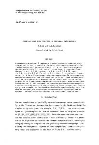
We now turn our focus to poset data structures. A poset data structure is a generalpurpose data structure that records the elements and relations of a poset. We begin with a straightforward matrix implementation in Section 5.1, continue with Siena poset in Section 5.2 and finish with ChainMerge in Section 5.3. The order was chosen so that each structure is more complex than the previous one. Later in Section 6 we discuss poset-derived forest which is a special-purpose data structure that stores a subset of the relations of a poset. Figure 2 contains representations of all three data structures studied in this section.

5.1

Incidence matrix

A poset can be represented as a directed acyclic graph (DAG) where the vertices correspond to the elements of the poset and the edges correspond to the relations between the elements. Specifically, if there exists a path from vertex a to b, then a dominates b. An incidence matrix is a straightforward implementation of a DAG. An incidence matrix for a poset with n elements is an n × n matrix where the cell (a, b) stores information about the relation of the element on row a to the element in column b. In Figure 2a we use X in cell (a, b) to denote that the element on row a dominates the element in column b. Obviously, if cell (a, b) contains X then cell (b, a) cannot contain X. The space complexity of an n × n matrix is Θ(n2 ). We present two similar variants: the matrix and the query-optimized matrix (q-o

9

1

6

5

2

3

7

4

1

7 6

5

X

X

X

X

2

3

X

7

X

3

6

5

2

1

4

X

X

X

X

X

X

4

(a) Matrix. X in cell (a, b) indicates the

(b) Siena poset. a → b indicates a domi-

element on row a dominates the element

nates b. Note that the relation 7 2 for

in column b.

example is implicit.

A -1-

B --2

3

---

C 00-

6

--1

7

1-2

5

--4

(c) ChainMerge.

A, B, and C are the

chains. The numbers on the top left corner of each element indicate the index of the highest element of each chain, starting from 0, that this element dominates.

Figure 2: Three poset data structures with the same data. Root elements are shown as filled in each of the figures.

10 matrix). The variants differ only in the add operation: whereas the matrix compares a new element to every existing element (thus resulting in linear query complexity growth), the query-optimized matrix uses existing information to deduce the relation of the new element to the existing elements. The query-optimized matrix variant has very good query complexity but worse total complexity. Algorithm 1 is the regular matrix add operation. The algorithm inserts the new element into the Matrix and updates the rest of the matrix to reflect the fact. The algorithm compares the new element with each existing element resulting in O(n) query complexity and O(n) total complexity. Algorithm 2 deletes an element from the Matrix and updates the relations accordingly. This requires touching every remaining element in the matrix which results in O(n) total complexity. No oracle queries are performed resulting in O(1) query complexity. The query-optimized matrix add variant is presented in Algorithm 3. The algorithm avoids doing unnecessary oracle queries by exploiting the information already gathered during the insertion process to the extent possible. If the algorithm detects that an existing element e dominates the new element it scans the matrix to find elements that dominate e and updates their relation to the new element without performing additional oracle queries. Likewise, if the algorithm detects the new element dominates an existing element e it scans the matrix to find elements dominated by e and updates their relation to the new element. Because of the extra scans, the algorithm has a worst-case total complexity of O(n2 ). The worst-case query complexity of the algorithm is O(n) as is the case with the regular add variant, although benchmarks show that the query-optimized matrix add variant performs considerably better in practice. Algorithm 4 computes the root set of the Poset using the information recorded in the Matrix. The algorithm scans the entire matrix which results in O(n2 ) total complexity. Query complexity of the algorithm is again O(1) since no element comparisons are performed. Algorithm 5 performs a look-up using the information recorded in the Matrix. It has a total and query complexity of O(1). A note on pseudo code notation: Pdominates[r,c] denotes a look-up of the value on row r and column c in the matrix. Pdominates[r,c] = true means that element r dominates element c.

11

5.2

Siena filters poset

Siena filter poset is a DAG-like poset used in the Siena project [CRW01], discussed previously in Section 3.1. For each node in the Siena poset, successor and predecessor sets are maintained. Insertion and deletion are straightforward. Worst-case space complexity of Siena is O(n2 ). Siena is limited in terms of scalability [TK06]. Posetderived forest is an adaptation of Siena that was designed for fast addition, deletion, and root set computation. We study poset-derived forest in detail in Section 6. We describe add, delete, look-up, and root set algorithms for the Siena poset data structure [CRW01]. Siena authors have not published a description of the algorithms but the Siena project Java code is publicly available [Car12]. We used the actual Siena project code and a description of the algorithms by Tarkoma and Kangasharju [TK06]. Algorithm 7 adds an element into the Siena poset. The necessary helper functions are listed in Algorithm 8. The algorithm first traverses the poset in breadth-first order starting from the root to find the predecessors of the new node. Then it traverses the poset starting from the predecessors set to find the successors of the new node. The successor set must be pruned. It is possible that a node in the successor set is also an ancestor of another node in the successor set. After pruning the algorithm uses the predecessor and successor sets obtained to insert the new node into the poset at the correct position. Finding the predecessor and successor sets results in O(n) query complexity. Looping through all successors for each predecessor results in O(n2 ) total complexity. Note that the choice of breadth-first order for the add algorithm is not arbitrary. Depth-first order could be used but breadth-first order results in better performance both in terms of number of oracle queries and amount of CPU time used because the depth-first variant would have to prune the predecessor set as well. Using breadthfirst order ensures that the predecessor set contains only the direct predecessors of the new node. Algorithm 9 deletes an element from the Siena poset. When an element is deleted, its successors’ predecessor sets and its predecessors’ successor sets must be updated accordingly. If the deleted element was a root element, its successor elements with an empty predecessor set become new root elements. If the deleted element was not a root element, each successor is connected to each predecessor unless the predecessor in question is already an ancestor of that successor. The worst-case estimate for

12 both the number of successors and predecessors is n. In addition, the ancestor check has to traverse at most n elements. This yields a total complexity of O(n3 ). Since no direct element comparisons are done, the query complexity of the algorithm is O(1). Root set computation is trivial: because the root set elements are the root nodes of the structure, they can be obtained without any extra computation. Because of the triviality of the operation, we did not include pseudo code for it. Total complexity of Siena root set computation is O(w). The query complexity is O(1). Algorithm 6 performs a look-up operation using the information stored in the Siena poset. Let us compare elements a and b. The algorithm first checks whether a is an ancestor of b. If that is the case, a dominates b and the algorithm terminates. If that is not the case, the algorithm checks whether b is an ancestor a. If b is an ancestor of a, b dominates a. Otherwise a and b are incomparable. The ancestor checks visit at most n elements resulting in O(n) total complexity. Since no oracle queries are performed, the query complexity is O(1).

5.3

ChainMerge

ChainMerge is a data structure by Daskalakis et al [DKM+ 11]. It stores the poset as a chain decomposition with domination information stored at each element. Specifically, each element stores the highest element it dominates in every other chain. This results in Θ(wn) space complexity if the chain decomposition is minimum and Θ(wmax n) space complexity if the chain decomposition is not minimum. We will return to this issue later in the section. This section is organized as follows. In Section 5.3.1 we study offline insertion algorithm by the ChainMerge authors. In Section 5.3.2 we present our online adaptation of an offline insertion algorithm by the ChainMerge authors. In Section 5.3.3 we present our delete algorithm and the ChainMerge authors’ look-up algorithm. Both algorithm are relatively simple and are thus presented together. In Section 5.3.4 we present our root set computation algorithm and finally in Section 5.3.5 and Section 5.3.6 we discuss ways to maintain a minimum chain decomposition.

13 5.3.1

Offline insertion algorithms

Unlike the Siena poset, which was designed for content filtering, ChainMerge was devised as an aid in sorting and selection. The insertion algorithms presented by the ChainMerge authors are therefore offline algorithms, i.e. they require that the set of input elements is known in advance. The POSET-MergeSort algorithm by Daskalakis et al [DKM+ 11] constructs a ChainMerge structure by recursively partitioning the set of input elements into smaller parts. The POSET-BinInsertionSort algorithm by the same authors is more suitable for the online insertion case since it processes the input elements one at a time. POSET-BinInsertionSort in its original form does however require that the width w of the constructed poset is known in advance which is not possible without knowing the input elements. We will present an online version of the POSET-BinInsertionSort algorithm without this requirement in Section 5.3.2. POSET-BinInsertionSort works by maintaining a chain decomposition of the partially constructed poset into w chains where w is an upper bound on the width of the fully constructed poset. When a new element is inserted, its relation to every other element is determined by executing 2w binary searches to find the smallest element in each chain that dominates the new element and the largest element in each chain that is dominated by the new element. This results in O(w log n) query complexity which is worse than the lower bound of Section 4.3 by a factor of w. Daskalakis et al present a query-optimal modification of POSET-BinInsertionSort called EntropySort that achieves the theoretical lower bound by exploiting the properties of the partially constructed poset to turn the binary searches into weighted binary searches. The weights are assigned so that the number of oracle queries required to insert an element into a chain is proportional to the number of candidate posets that are eliminated by the insertion of that element [DKM+ 11]. This requires computing the number of width-w extensions (the candidates) of the partially constructed poset for each input element, which is too expensive in practice. We do not consider EntropySort further. 5.3.2

Online insertion algorithm

We present an online adaptation of the POSET-BinInsertionSort algorithm by Daskalakis et al [DKM+ 11]. The original algorithm maintains a chain decomposition

14 of width at most w and has O(w log n) query complexity. The exact mechanism for maintaining the chain decomposition is left unspecified since Daskalakis et al present the POSET-BinInsertionSort and EntropySort algorithms more as exercises in query optimality rather than practical algorithms. Although we do not know the width of the final poset, w, in the online case, it is possible to maintain a chain decomposition of size wc where wc is the width of the current poset rather than the width of the final poset. Since wc ≤ w, such a version of the algorithm would also have O(w log n) query complexity, although maintaining a minimum chain decomposition is very expensive in practice. We delay discussion of the minimum chain decomposition case until Section 5.3.5. We now present the online adaptation of the POSET-BinInsertionSort algorithm. This version of the algorithm does not maintain a minimum chain decomposition. Rather, it maintains a chain decomposition of width at most wmax . The algorithm does this by inserting the new element into the longest suitable chain. If no suitable chains are found, it creates a new chain for the element. Once an element is inserted into a chain, it is never moved to another chain. In this sense our algorithm is analogous to a first-fit algorithm. A first-fit algorithm would always choose the first suitable chain whereas our algorithm chooses the longest suitable chain in order to better exploit binary search. Finding the longest suitable chain does not incur any extra cost because the relation of the new element to every chain must be determined in any case. The online POSET-BinInsertionSort algorithm performs 2wmax binary searches to determine the relation of the new element to the existing elements, which results in O(wmax log n) query complexity. Since w(P) ≤ wmax (P), this is worse query complexity than the query complexity of the original algorithm. We present a way to reach O(w log n) query complexity in Section 5.3.5. Total complexity of the online algorithm is O(wmax log n+n) The additional O(n) in total complexity is the cost of updating the relations of existing elements to reflect the newly inserted element. See Algorithm 10 for a pseudo code representation of the algorithm. Let us finally show why maintaining a minimum chain decomposition is “harder” than maintaining a chain decomposition of an arbitrary size. Let elements a, b, c, d, e, f, and g be input elements to a first-fit algorithm and let them have the relations shown in Table 1.

15 a a

b

c

X

X

b

d

e

f

X

X

X

g

X

c d e

X

X X

X

X X

X

f g

X

Table 1: Example relations. X in cell (a, b) indicates the element on row a dominates the element in column b. If the elements are inserted in alphabetical order, after inserting f we have two chains: a b c and d e f . When g is inserted, the algorithm is forced to create a new chain for g. It cannot insert g to the first chain because b g and it cannot insert g to the second chain because g f . If the insertion order would have been a, e, c, d, b, f, g instead, after c was inserted we would still have only one chain, namely a e g c. After f was inserted we would have one other chain, namely d b f . The second insertion order resulted in a chain decomposition with one less chain, which is also a minimum chain decomposition. The algorithm failed to produce a minimum chain decomposition because of an unfavorable insertion order. In fact, it has been shown that an adversary can “trick” a first-fit algorithm into decomposing a poset of width 2 with n elements into n chains by carefully choosing the input order of the elements [BKS10]. 5.3.3

Delete and look-up algorithms

No known ChainMerge delete algorithm exists. Algorithm 11 is our algorithm for deleting a single element. We use e to denote the deleted element and echain to denote the chain e belonged to. The implementation is straightforward: First the algorithm removes the element e. If the removed element was the only element in its chain, the chain is removed too. Then the algorithm iterates over the remaining elements to update their domination information for the chain echain . If the entire chain was removed, the domination information is set to nil. Otherwise it is sufficient to subtract one from the index of the largest element each element dominates in chain echain , if the current value for echain is larger than the index of the deleted element,

16 eindex . If the current value for echain is smaller than eindex , nothing needs to be done since the deletion could not have affected the value. The algorithm runs in O(n) time with O(1) query complexity. Algorithm 12 is a look-up algorithm by Daskalakis et al [DKM+ 11]. It uses the information stored in the poset to determine the relation of the elements and runs in O(1) time with O(1) query complexity. 5.3.4

Root set computation

We begin with some useful results. Definition 5.1. Maximal element of a chain C ⊆ P is an element e ∈ C such that e ei for all ei ∈ C, ei 6= e. Lemma 5.2. If an element is dominated by an element in another chain, it is also dominated by the maximal element of that chain. Conversely, if an element is not dominated by the maximal element of a chain, it is not dominated by any element in that chain. Proof. Let C1 ⊆ P and C2 ⊆ P be chains of poset P. Let e1 ∈ C1 and e2 ∈ C2 be elements of the poset. First part: Let us assume e1 e2 . The claim is trivially true if e1 is the maximal element of chain C1 . If e1 is not the maximal element of C1 there must be a maximal element emax ∈ C1 such that emax e1 . From transitivity of the relation it follows that if emax e1 and e1 e2 then emax e2 . Second part follows from the first part. Theorem 5.3. An element is part of the root set if and only if it is the maximal element of its chain and not dominated by the maximal element of any other chain. Proof. 00 ⇒00 : Let us assume er ∈ P is part of the root set for poset P. Therefore it must be true that ei er for all ei ∈ P, ei 6= er . If the element er ∈ C is not the maximal element of its chain, there exists a maximal element emax ∈ C such that emax er which leads to a contradiction. Likewise, the existence of an element e1 ∈ C1 in another chain C1 such that e1 er leads to a contradiction. 00

⇐00 : Let er ∈ C be the maximal element of chain C that is not dominated by the maximal element of any other chain. By definition there is no element e ∈ C such that e er . Based on Lemma 5.2 and our premise we can conclude that there is no element e ∈ Ci for all Ci ⊆ P, Ci 6= C such that e er . Therefore e er is true for all e ∈ P and thus er is part of the root set.

17 Algorithm 13 is our algorithm for computing the root set of the ChainMerge poset. The algorithm considers the first element of each chain as a potential root element and discards it if it is dominated by another potential root element. The correctness of the algorithm follows from Theorem 5.3. The algorithm visits w chains w times resulting in O(w2 ) total complexity with O(1) query complexity. 5.3.5

Maintaining a minimum chain decomposition

As seen previously, a chain decomposition of a poset constructed by a first-fit or equivalent algorithm might be considerably larger than the width of the poset. We will show in Section 7 that unless minimizing the number of oracle queries is paramount, our first-fit algorithm is actually a better choice than an algorithm that aims to maintain a minimum chain decomposition. We will next discuss ways to maintain a minimum chain decomposition for the sake of completeness. There are two approaches to the issue: the algorithm can constantly maintain a minimum chain decomposition or it can periodically restructure the chain decomposition. An algorithm that constantly maintains a minimum chain decomposition is an online chain decomposition algorithm. Known online chain decomposition algorithms assume the linear extension hypothesis, which postulates that each new element is maximal in the poset at the time of insertion, i.e. that the new element is not dominated by any elements already in the poset [IG]. Considering the use cases we have presented so far, we can not accept the linear extension hypothesis and must therefore settle for an offline chain decomposition algorithm. Several offline chain decomposition algorithms exist. We will present the Merge algorithm by Tomlinson and Garg [TG97] in the next section. Merge operates on a set of chains that represent a not necessarily minimal chain decomposition of a poset making it ideal to use with ChainMerge. Other offline chain decomposition algorithms are Reduce by Bogart and Magagnosc [IG] and Peeling by Daskalakis et al [DKM+ 11], which is similar to Merge. We did not choose Reduce because it was outperformed by Merge in comparisons done by Ikiz and Garg [IG]. Peeling on the other hand requires us to know the width of the poset in advance. It also requires that the cardinality of the input structure is at most 2w [DKM+ 11] which we cannot guarantee.

18 5.3.6

The Merge algorithm

Tomlinson and Garg present Merge as part of the solution to finding an antichain. It follows from Dilworth’s theorem that an antichain of size at least k exists if and only if the poset cannot be partitioned into k − 1 chains [TG97]. Given a chain decomposition with n chains, their FindAntiChain algorithm tries to partition the poset into k − 1 chains by calling Merge repeatedly to reduce the number of chains. If a chain decomposition with k − 1 chains is found, an antichain of size at least k does not exist. Each successful invocation of Merge reduces the number of chains in the chain decomposition by one. Merge takes as input a list of queues sorted in ascending order which represent the chains of the chain decomposition. Merge works by iterating over the head (smallest) elements of the input queues until one or more input queues become empty (in which case the merge will succeed) or until no head elements are comparable (in which case the merge failed). Each iteration compares the head element in every input queue to the head element in every other input queue. If the elements are comparable, the dominated element is removed from the input queue and appended to an output queue. The incomparable elements form an antichain A and are not compared against each other on subsequent iterations. Note that the existing ChainMerge structure can be used to determine the relations of the elements and therefore no oracle queries are required, which results in O(1) query complexity. Pseudo code for Merge is presented in Algorithm 15. In the pseudo code variable ac keeps track of the currently formed antichain, move keeps track of the elements to be moved, and bigger keeps track of the relations of the elements. G is a queue insert graph. It can be initially any acyclic graph with k − 1 edges. For an input with n input queues, Pi , there are n − 1 output queues, Qi . The crucial part is deciding to which output queue an element is placed. It is shown that by making an incorrect choice at this step the algorithm may run out of options with later elements [TG97]. Merge works by maintaining a queue insert graph, which is a connected acyclic graph, i.e. a tree. The n vertices of the graph correspond to the n input queues while the n − 1 edges correspond to the n − 1 output queues. We use Glabel(i,j) to denote the label of an output queue that corresponds to an edge between vertices i and j and Pi to denote the input queue that corresponds to the vertex i. An edge between vertices i and j means that the head elements of Pi and Pj dominate the tail (largest) element of Q( i, j).

19 The following is a description of the FindQ algorithm by Tomlinson and Garg [TG97]. The algorithm uses the queue insert graph to find an appropriate output queue for an element. When the head element of Pi is dominated by the head element of Pj , an edge i, j is added to the graph. Since the graph was a tree, it now contains exactly one cycle which includes the edge i, j. Let i, k be the other edge incident to i that is part of the cycle. The algorithm now removes i, k and assigns the label Glabel(i,k) to i, j. The element is placed to the output queue denoted by that label. The pseudo code for the FindQ algorithm is listed in Algorithm 14. If the size of the antichain A reaches the size of the chain decomposition while iterating over the elements, the merge fails and the algorithm terminates. If one of the input queues becomes empty, the merge will succeed and the algorithm appends the rest of the input queues to the appropriate output queues before terminating. Tomlinson and Garg do not describe the append step in more detail. The following is a description of our simple although suboptimal append algorithm. The algorithm FinishMerge assigns each of the n − 1 output queues to the at most n − 1 non-empty input queues so that each non-empty input queue is assigned exactly one output queue. First, we observe that based on the previous description of the queue insert graph, the remaining elements of an input queue denoted by vertex i in G may be appended to any of the output queues denoted by edges labeled with Glabel(i,j) , 1 ≤ j ≤ n, that is any edge incident to i. The algorithm first finds all vertices that represent non-empty input queues with exactly one edge connecting them to the rest of the graph and assigns the only possible output queue to each of them. The assigned edges are removed from the graph. Removal of the edges results in vertices with previously two edges now having only one edge. The algorithm repeats until all output queues are assigned. Because the algorithm does not consider empty input queues, it is sometimes left with several non-empty input queues that have more than one edge incident to them but no non-empty input queues with only one edge incident to them. In that case the algorithm chooses one of the input queues and assigns it an output queue. This makes the algorithm slightly suboptimal for it is possible to make a non-optimal choice at this point. The deviation from minimum chain decomposition is not large as seen later in Figure 11 in Section 7. Pseudo code for the FinishMerge algorithm is presented in Algorithm 14. Finally, the Minimize algorithm of Algorithm 14 ties it all together by repeatedly calling Merge to reduce the size of the chain decomposition. Minimize differs from

20 Tomlinson and Garg’s FindAntiChain algorithm in that Minimize calls Merge for the entire chain decomposition until merging no longer succeeds. FindAntiChain on the other hand calls Merge for a rotating subset of the chains based on the value of k which is the size of the antichain the algorithm is trying to find [TG97]. Let us next estimate the worst-case total complexity of Minimize. The loop in Minimize is executed at most wmax − w times which equals n in the worst case. The Merge function inside the loop consists of a while loop, two nested for loops inside the while loop, a move loop inside the while loop, and a FinishMerge call. The while loop in Merge is executed at most n times and both for loops at most wmax times. The move loop is executed at most n times. The cycle finding algorithm inside the move loop visits all nodes of G in the worst case which results in O(nwmax ) total complexity for the move loop. Based on the above, the 2 + nwmax )). The FinishMerge total complexity of the while loop is O(n(wmax algorithm repeatedly iterates through the vertices of G so that on each iteration at least one vertex (input queue) is assigned an edge (output queue) which re2 ) total complexity for FinishMerge and together with the while sults in O(wmax 2 2 loop complexity in O(n(wmax + nwmax ) + wmax ) total complexity for Merge and 2 2 2 O(n (wmax + nwmax ) + nwmax ) total complexity for Minimize. We have neglected one cost so far. After the chain decomposition has been minimized, the relation of each element to other chains has to be re-established. This is equivalent to re-adding each of the elements to the structure with one exception: the query complexity is constant this time because the existing CM structure can be used for element comparisons. The same is true for the Minimize operation which makes the query complexity of the entire reconstruction operation O(1). The total complexity of the reconstruction operation is the total complexity of Minimize and the cost of n add operations where n is the number of elements in the poset. One last thing to discuss is the interval, in terms of the number of elements inserted, between successive reconstruction operations. As the total complexity estimate suggests, unless keeping the number of oracle queries low is paramount (or the input data is known to be pathological), reconstructing the chains is most likely not worth the time spent doing it. If the number of oracle queries must be kept low at all costs, reconstructing the chains often—even after every insertion—is the best choice. We experiment with a few possible values in Section 7.

21 Structure

add

delete

roots

look-up

Siena poset

O(n)

O(1)

O(1)

O(1)

ChainMerge

O(wmax log n)

O(1)

O(1)

O(1)

ChainMerge

O(w log n)

O(1)

O(1)

O(1)

Matrix

O(n)

O(1)

O(1)

O(1)

Q-o Matrix

O(n)

O(1)

O(1)

O(1)

Ω(w log n)

Ω(1)

Ω(1)

Ω(1)

min. chains

Lower bound

Table 2: Query complexities. Structure

add

delete

roots

look-up

space comp.

Siena poset

O(n2 )

O(n3 )

O(w)

O(n)

O(n2 )

ChainMerge

O(wmax log n + n)

O(n)

2 ) O(wmax

O(1)

Θ(wmax n)

2

O(w log n + n)

O(n)

O(w )

O(1)

Θ(wn)

Matrix

O(n)

O(n)

O(n2 )

O(1)

Θ(n2 )

Q-o Matrix

O(n2 )

O(n)

O(n2 )

O(1)

Θ(n2 )

Lower bound

Ω(n)

Ω(n)

Ω(w)

Ω(1)

Ω(wn)

ChainMerge min. chains

Table 3: Total complexity of the operations and space complexity. For structures other than Siena the lower and upper bounds on space requirement are the same.

5.4

Worst-case complexities

Tables 2 and 3 compare the data structures in terms of query complexity and total complexity. Table 3 contains also space complexity estimates. For structures other than Siena the lower and upper bounds on space requirement are the same and they are thus denoted by theta (Θ) instead of big-oh. The minimum chains ChainMerge variant is the smallest of the data structures studied in this section with a space complexity of O(wn). Since w = n in the worstcase and n2 /4 + O(n) ∈ O(n2 ), our findings are in line with the theoretical lower bound of Section 4.3. It must be noted, though, that none of our structures are especially space efficient. We will discuss space efficient poset structures briefly in Section 5.5. The data structure with least oracle comparisons is also the minimum chains Chain-

22 Merge variant with a query complexity of O(w log n). Since w = 1 represents a total order, our query complexity is worse than Ω(log n+w) of Section 4.3 with all possible values of w. The EntropySort algorithm discussed previously is query-optimal but too expensive in practice.

5.5

Other data structures

We will briefly mention two other poset data structures before moving forward. The purpose of both structures is to reduce the size of the stored poset. Since we are not particularly concerned with space efficiency, we will not consider these data structures further. Bit-encoded ChainMerge by Farzan and Fischer [FF11] reduces the size of a poset by storing the transitive reduction of a graph G representing the poset and not G itself. Transitive reduction of G is the smallest subgraph of G with a transitive closure equal to the transitive closure of G [FF11]. Furthermore, the chains of the poset and their relations are stored as bit vectors. The main advantage of bit-encoded ChainMerge is the smaller space requirement although the structure is applicable only to posets of small width. The space requirement of a bit-encoded ChainMerge structure is (1 + )n log n + 2nw(1 + o(1)) bits for an arbitrary small constant > 0 [FF11], which is greater than the theoretical lower bound of Section 4.3. Munro and Nicholson [MN12] present their own bit-encoded data structure for arbitrary posets that matches the theoretical lower bound of Section 4.3. Munro and Nicholson’s data structure is an example of a succinct data structure. A succinct data structure matches the theoretical lower bound on the size of the structure to within lower order terms while supporting efficient query operations [MN12].

6

Poset-derived forest

Poset-derived forest (PF) by Tarkoma and Kangasharju is a data structure designed for fast additions, deletions, and fast computation of the root set [TK06]. Posetderived forest achieves these fast operations by storing only a subset of the relations of a poset. Figure 3 illustrates the difference between Siena poset and poset-derived forest. Because complete relations are not stored, look-up is not a meaningful operation for poset-derived forest, and we substitute it with computing the covered set. With incomplete relations, deletion can no longer be performed with O(1) query

23 complexity. Nevertheless, PF performs considerably better than Siena poset in the tasks it was designed for. We provide brief comparison of PF against Siena poset in Section 7.5. For a more comprehensive comparison of PF against Siena poset the reader is referred to the paper by Tarkoma and Kangasharju [TK06]. We begin with a few crucial definitions in Section 6.1 and describe the basic PF algorithms in Section 6.2. In sections 6.3 to 6.5 we discuss several variants of the basic PF structure. Tables 4 and 5 provide a summary of the query and total complexities of the variants. The variants are benchmarked in Section 7.5.

6.1

Definitions

These definitions are based on the definitions by Tarkoma and Kangasharju [TK06]. Definition 6.1. Poset-derived forest is a pair (P, 3) where P is the set of elements and 3 is an irreflexive, transitive binary relation. For each element a ∈ P , there exists at most one element b ∈ P such that a 3 b. If a 3 b then a b. The elements a ∈ P for which there does not exist an element b ∈ P such that b 3 a form the root set. The elements of the root set can be thought of as children of a so-called imaginary root which is a node not in P . Including the imaginary root allows treating the entire forest as a single tree. Definition 6.2. A poset-derived forest is sibling pure at node a if all children of a are mutually incomparable. A poset-derived forest is sibling pure if it is sibling pure at every node, including the imaginary root. Generally, we do not consider non-sibling-pure forests in this thesis, although there may be use cases in content-based routing that do not require sibling purity [TK06]. The lazy-evaluated poset-derived forest variants of Section 6.4 are a special case: they are sibling pure only to a certain depth.

6.2

The algorithms

We describe algorithms for the poset-derived forest data structure. All algorithms except covered set computation are originally described by Tarkoma and Kangasharju [TK06]. We do not provide pseudo code for the root set algorithm because it is trivial.

24 7

5

3

6

1

4

2

Figure 3: Removing the dotted relations of this Siena poset produces one of the many possible poset-derived forests for this poset. The filled node is a root node. Algorithm 16 adds a new element to the poset-derived forest. The algorithm traverses the forest starting from the imaginary root until a node is found that dominates the new element. The new element then becomes the child of that node. At each node, if the new element dominates any children of the node, the dominated children become the new element’s children. If the new element is not dominated by any existing nodes, it simply becomes a root node. In the worst case, every node is visited before the algorithm terminates resulting in O(n) total complexity and O(n) query complexity. The call to the Balance function on line 33 in Algorithm 16 is only done for the actively balanced variant, discussed in Section 6.3. Algorithm 17 deletes an element from the poset-derived forest. It runs the Add algorithm for every subtree rooted at the deleted element. In the worst case, there are n subtrees resulting in O(n2 ) total complexity and O(n2 ) query complexity. Running Add for the subtrees is necessary to maintain sibling purity. We do not discuss cases where sibling purity is not maintained. Algorithm 18 performs covered set computation. The algorithm traverses the entire structure resulting in O(n) query and total complexities. Root set computation is trivial. Every non-covered filter is a root node in a maximal (i.e. sibling pure) posetderived forest [TK06]. Thus it is sufficient to list the root nodes of a poset-derived forest to obtain the root set which results in O(w) total complexity and O(1) query complexity.

25

6.3

Balanced PF

We present two alternative balancing implementations for the poset-derived forest, called active balancing and passive balancing. These balancing schemes are not related to interface-based balancing discussed by Tarkoma and Kangasharju [TK06]. Passive balancing balances the structure by always inserting a new element into the shortest subtree. Active balancing extends passive balancing by doing additional rebalancing operations. Active balancing results in shorter trees but requires more oracle queries due to the rebalancing operations. We compare the performance of balanced PF variants in more detail in Section 7.5. The passive balanced variant always inserts the new element into the shortest possible subtree. It achieves this by storing the height of the tallest subtree rooted at each node. Whereas the basic PF Add operation of Algorithm 16 makes an arbitrary choice of the subtree to descend to at each node—seen as the assignment to next on line 17 of Algorithm 16—the passive balanced variant simply chooses the shortest subtree. We do not present pseudo code for this fairly trivial variant. Passive balancing can fail to produce the shortest possible structure because it does balancing only by choosing the subtree when traversing the poset-derived forest. In the worst case the input values are inserted in increasing order and no choosing is done. Active balancing on the other hand constantly monitors the height of the subtrees and rebalances them. Active balancing does a rebalancing operation after each inserted element. This is seen as the call to the Balance function on line 33 in Algorithm 16. Algorithm 19 contains the pseudo code listing for the Balance algorithm. The balancing algorithm works as follows. First the algorithm determines whether the difference in length of the shortest and tallest subtree rooted at node r exceeds a certain threshold. The threshold calculation can be seen on line 5 in Algorithm 19. The point of the threshold calculation is to ensure that the balancing operation is meaningful. In the worst case the taller subtree is appended to the end of the shorter subtree. The algorithm therefore ensures that the combined length of the subtrees is 2 less than the original length. If the threshold is exceeded, the algorithm traverses the longer subtree recursively to find the nodes at the middle of the subtree and moves them to the shorter subtree if possible. The total and query complexities of the Balance function are O(n). Because the Balance function is called from the end of the Add function, it brings the total and query complexities of the Add function to

26 O(n2 ) for the actively balanced variant.

6.4

Lazy-evaluated PF

Lazy-evaluated poset-derived forest works by postponing the evaluation of elements until necessary. The lazy-evaluated variant has a predetermined initial evaluation depth to which it evaluates the elements. For example, when a new element is inserted into a lazy-evaluated PF with initial evaluation depth of one, the new element’s relation to the root nodes is determined in the usual manner. After this step the new element either becomes a root node itself or a child of one. The evaluation stops after this step. The structure is sibling pure to depth 1. Evaluation to a depth of at least 1 is necessary for fast root set computation. Each node of the lazy-evaluated PF contains an evaluated? flag which indicates whether the children of the node are evaluated. The flag is necessary because each subtree of the structure might be evaluated to a different depth. Although the initial evaluation depth is fixed, insertion of a new root node causes the evaluation depth of the subtrees rooted at the new root node grow by one as seen in Figure 4. Node 31 in the figure dominates all other nodes and node 15 dominates nodes 7 and 3. In Figure 4a element 31 is inserted first and the resulting structure is evaluated to depth 1. In Figure 4b element 31 is inserted last. Because the subtree rooted at 15 is already evaluated to depth 1, the final subtree of Figure 4b is evaluated to depth 2. Although varying evaluation depth makes the implementation more complex, a simplified implementation does not justify discarding already computed information. Another noteworthy thing in Figure 4 is that a lazy-evaluated PF contains considerably more leaf nodes than an ordinary PF. This is beneficial since the deletion of a leaf node is cheaper than the deletion of a non-leaf node because it does not require relocating the deleted node’s children. On the other hand, deletion of a root node is more expensive in the lazy evaluated variant because the replacement root node is not immediately known. There is a trade-off between smaller and larger evaluation depths; smaller evaluation depths result in more efficient add operation but less efficient delete operation than larger evaluation depths. The insertion algorithm for the lazy-evaluated PF variant is a simple modification of Algorithm 16. When the initial evaluation depth is reached (or when a subtree with an unevaluated root node is encountered), the new value is inserted at the current position. The delete operation does not require any modification to Algorithm 17

27 31

31

15

7 (a) 31 inserted first

15

3

7

3

(b) 31 inserted last

Figure 4: The same lazy-evaluated PF with an initial evaluation depth of 1 and two different insertion orders. The dotted line indicates an unevaluated node. since it already calls add for the children of the deleted node.

6.5

PF merging

If the use case is insertion-heavy, it may be beneficial to first construct smaller poset-derived forests and then merge them. We call such a structure MergeForest. A straightforward MergeForest implementation uses an array of n poset-derived forests. When a new element arrives, it is inserted into the next PF in a roundrobin fashion. A merge step involves merging all n − 1 PFs to the nth PF. Merging of two poset-derived forests, P F1 and P F2 , is accomplished by inserting each of the trees in P F2 to P F1 with the ADD function of Algorithm 16. We will see in Section 7 that this approach will spare a considerable amount of oracle queries in the ideal case. This is possible because the merge step benefits from adding entire subtrees by comparing only the root element and does not therefore require nearly as many oracle queries as inserting into the smaller posets spared. Another issue, which we will not pursue further, is that the construction of the smaller posets could be done in parallel with a multi-CPU computer or in a distributed manner with a workload distribution framework such as MapReduce [DG08]. One of the issues with a real production scale system would be how to share the data (i.e. pieces of the forest) with other nodes. Salo [Sal10] has studied a similar issue in the context of content-based routing.

28 Structure

add

delete

roots

Basic PF

O(n)

O(n2 ) O(w)

covered set space complexity

2

O(n)

O(n)

Balanced PF (passive)

O(n)

O(n ) O(w)

O(n)

O(n)

Balanced PF (active)

O(n2 ) O(n3 ) O(w)

O(n)

O(n)

2

Lazy PF

O(n)

O(n ) O(w)

O(n)

O(n)

Lower bound

Ω(n)

Ω(n2 )

Ω(n)

Ω(n)

Ω(w)

Table 4: Poset-derived forest and variants total complexities. Structure

add

delete

roots

covered set

Basic PF

O(n)

O(n2 )

O(1)

O(n)

Balanced PF (passive)

O(n)

O(n2 )

O(1)

O(n)

2

3

Balanced PF (active)

O(n ) O(n )

O(1)

O(n)

Lazy PF

O(n)

O(n2 )

O(1)

O(n)

Lower bound

Ω(n)

Ω(n2 )

Ω(1)

Ω(n)

Table 5: Poset-derived forest and variants query complexities.

7

Experimental evaluation

Let us turn our focus to experimental evaluation of the data structures and algorithms we presented in previous sections. First we describe the benchmarking setup in sections 7.1 to 7.3. Then we present the results for poset structures in Section 7.4 and for poset-derived forest in Section 7.5.

7.1

Input values

We used simple integer values as the inputs and their natural order as the order of the elements of a poset. To introduce artificial incomparability among the elements we used several different comparability percents. A comparability percent for a benchmark run determines the percentage of mutually comparable elements in the set of input values. The comparabilities were distributed uniformly among the set of input values as described in Section 7.2. We used the following comparability percents: 0, 25, 50, and 85. A comparability percent of 50 is a reasonable value when the actual use case for the poset is not known. The zero percent case is hardly encountered in practice but was included

29

ChainMerge: Query complexity

Oracle queries

4000 3000 2000 1000 0 2000 1500 100

1000

75 50 Comp percent

Size of poset 500 25 0

0

Figure 5: Effect of comparability percent on the query complexity of the ChainMerge add operation.

Add: 0% comparability

Add: 25% comparability 2500

4000 Oracle queries

Oracle queries

3500 3000 2500 2000 1500 1000

2000 1500 1000 500

500 0

0 0

250

500

0

750 1000 1250 1500 1750 2000

250

500

Poset size

Poset size


2500

2000

Oracle queries

Oracle queries


2000 1500 1000 500 0

750 1000 1250 1500 1750 2000

1500 1000 500 0

0

250

500

750 1000 1250 1500 1750 2000

0

250

Poset size

Siena ChainMerge

500

750 1000 1250 1500 1750 2000 Poset size

Matrix Q-o Matrix

Figure 6: Number of oracle queries required for the add operation.

30 Add: 0% comparability

Add: 25% comparability 0.035

0.0014

0.03

0.0012

0.025 Seconds

Seconds

0.0016

0.001 0.0008 0.0006

0.02 0.015

0.0004

0.01

0.0002

0.005

0

0 0

250

500

750 1000 1250 1500 1750 2000

0

250

500

Poset size

Poset size



0.06

0.03

0.05

0.025

0.04

Seconds

Seconds

750 1000 1250 1500 1750 2000

0.03 0.02 0.01

0.02 0.015 0.01 0.005

0

0 0

250

500

750 1000 1250 1500 1750 2000

0

250

500

Poset size

750 1000 1250 1500 1750 2000 Poset size

Siena ChainMerge

Matrix Q-o Matrix

Figure 7: Amount of CPU time used per add operation.

Delete: 0% comparability


0.00014 0.00012 Seconds

Seconds

0.0001 8e-05 6e-05 4e-05 2e-05 0 0

0.00045 0.0004 0.00035 0.0003 0.00025 0.0002 0.00015 0.0001 5e-05 0 -5e-05

250 500 750 1000 1250 1500 1750 2000

0

250 500 750 1000 1250 1500 1750 2000

Poset size

Poset size


Delete: 85% comparability 0.0012

0.001

0.001

0.0008

0.0008 Seconds

Seconds

0.0012

0.0006 0.0004 0.0002

0.0006 0.0004 0.0002

0

0

-0.0002

-0.0002 0

250

500

750 1000 1250 1500 1750 2000 Poset size

Siena

0

250

500

750 1000 1250 1500 1750 2000 Poset size

ChainMerge

Matrix

Figure 8: Amount of CPU time used per delete operation.

31

Look-up: 0% comparability

Look-up: 25% comparability

0.000002

2.5e-05

0.000002 2e-05 Seconds

Seconds

0.000001 0.000001 0.000001 0.000001 0.000001

1.5e-05 1e-05 5e-06

0.000000 0.000000

0 0

250 500 750 1000 1250 1500 1750 2000

0

250 500 750 1000 1250 1500 1750 2000

Poset size

Poset size

Look-up: 85% comparability 7e-05 6e-05 5e-05 Seconds

Seconds

Look-up: 50% comparability 5e-05 4.5e-05 4e-05 3.5e-05 3e-05 2.5e-05 2e-05 1.5e-05 1e-05 5e-06 0

4e-05 3e-05 2e-05 1e-05 0

0

250 500 750 1000 1250 1500 1750 2000

0

250

500

Poset size

Siena

750 1000 1250 1500 1750 2000 Poset size

ChainMerge

Matrix

Figure 9: Amount of CPU time used per look-up operation.

Root set computation: 0% comparability


0.3

0.2

Seconds

Seconds

0.25

0.15 0.1 0.05 0 0

250

500

0.045 0.04 0.035 0.03 0.025 0.02 0.015 0.01 0.005 0

750 1000 1250 1500 1750 2000

0

250

500

Poset size

Poset size



0.03

0.02

Seconds

Seconds

0.025

0.015 0.01 0.005 0 0

250

500

750 1000 1250 1500 1750 2000 Poset size

Siena

750 1000 1250 1500 1750 2000

0.01 0.009 0.008 0.007 0.006 0.005 0.004 0.003 0.002 0.001 0 0

250

500

750 1000 1250 1500 1750 2000 Poset size

ChainMerge

Matrix

Figure 10: Amount of CPU time used per root set computation.

32 CM: Add: 25% comparability

Oracle queries

Number of chains

CM: Number of chains: 25% comparability 450 400 350 300 250 200 150 100 50 0 0

250

500

2000 1800 1600 1400 1200 1000 800 600 400 200 0

750 1000 1250 1500 1750 2000

0

250

500

750 1000 1250 1500 1750 2000

Poset size

Poset size

CM: Number of chains: 50% comparability

CM: Add: 50% comparability 1600 1400

250

Oracle queries

Number of chains

300

200 150 100 50

1200 1000 800 600 400 200

0

0 0

250

500

750 1000 1250 1500 1750 2000

0

250

500

750 1000 1250 1500 1750 2000

Poset size

Poset size

CM: Number of chains: 85% comparability

CM: Add: 85% comparability

100

Oracle queries

Number of chains

120

80 60 40 20 0 0

250

500

750 1000 1250 1500 1750 2000

900 800 700 600 500 400 300 200 100 0 0

250

500

750 1000 1250 1500 1750 2000

Poset size

Poset size

CM: Add: 85% comparability 0.0008

0.0012

0.0007

0.001

0.0006 Seconds

Seconds

CM: Add: 25% comparability 0.0014

0.0008 0.0006

0.0005 0.0004 0.0003

0.0004

0.0002

0.0002

0.0001

0

0 0

250

500

750

1000

0

250

Poset size

ChainMerge ChainMerge-1

500

750

1000

Poset size

ChainMerge-50 ChainMerge-500

Figure 11: ChainMerge chain partition results. The figures on the left side represent the number of chains with different comparability percents and the figures on the right side represent the number of oracle queries for the same comparability percent. The two figures on the bottom represent CPU benchmarks. ChainMerge-1 reconstructs the chains after every insertion, ChainMerge-50 after every fifty inserted elements and so on.

33 because it induces worst-case behavior in many of the algorithms. 100 percent comparability represents a total order and is therefore outside the scope of this work, although we did want to bias the largest of the values towards a total order and thus chose 85 instead of 75 as the largest comparability percent. See Figure 5 for an example of the effect of comparability percent on query complexity. Most of the benchmarks were executed with uniformly distributed input values, i.e. each of the input values was as likely to be chosen as the nth input value to the benchmarked algorithm. In some cases the input values were fed to the benchmarked algorithm in strictly descending order.

7.2

Element comparison scheme

To introduce artificial incomparability among the elements a comparability matrix with uniformly distributed values was used. A comparability matrix records the comparability of each element to every other element in P . To compare elements a, b ∈ P we would first query the comparability matrix to find out whether a and b are comparable. If they are comparable, we would compare them by their natural order, i.e. if a > b then a b. The comparability matrix must satisfy two properties: symmetricity, i.e. a ∼ b ⇒ b ∼ a for all a, b ∈ P , and transitivity, i.e. a b ∧ b c ⇒ a c for all a, b, c ∈ P . Symmetricity is easily maintained by storing only half of the matrix as an upper triangular matrix and converting queries such as (5,2) to (2,5). Transitivity was ensured by running a transitivity checker after the matrix was constructed. The checker would detect and repair any transitivity violations found by adding missing relations to the matrix until it satisfied the transitivity requirement. Because of this step it was not feasible to estimate the resulting comparability percent of the matrix in advance. Rather, we constructed several matrices with different values for n and picked the ones that satisfied the required comparability percent. The entire process to produce a random set of comparabilities is as follows. First, the comparability matrix is filled with n values and then shuffled. Then the transitivity checker is run to enforce transitivity. After this the comparability percent of the resulting matrix is assessed. If the resulting comparability percent equals the requested percent within a 1% error margin, the algorithm terminates. Otherwise a new value for n is chosen and the process repeats. Binary search was used to find suitable values for n in a small number of steps.

34 Structure Siena poset

add

delete

2000/1000 1000/200

roots

look-up

dominated set

2000

10000

-

ChainMerge

2000

2000

20000

20000

-

Matrix

2000

2000

500

20000

-

Poset-derived forest

5000

5000

-

-

4000

Table 6: Batch sizes used for the CPU time benchmarks. A smaller batch size was used for 50% and 85% Siena add and delete benchmarks since they were very slow to execute compared to the other benchmarks.

7.3

Benchmarking setup

We implemented all data structures from scratch in Java. Although previous implementations of Siena posets and poset-derived forest are publicly available as part of the Siena [Car12] and Fuego [TKLR06] projects, a custom implementation guaranteed fair treatment of all data structures and allowed us to easily employ a custom element comparison scheme, which we described in Section 7.2. Our implementations of Siena poset and poset-derived forest are based on the description by Tarkoma and Kangasharju [TK06] and the Siena project Java implementation. The posetderived forest variant implementations are based on the original work in Section 6. Our ChainMerge implementation is based on the description by Daskalakis et al [DKM+ 11] and original work in Section 5.3. The rather trivial incidence matrix data structure is based on the description in Section 5.1. We used two different measures: the number of oracle queries required for an operation and the amount of CPU time used for an operation. For structures other than poset-derived forest, the number of oracle queries was measured only for the add operation since it is constant for the other operations. For poset-derived forest and its variants, we measured the number of oracle queries for the add and delete operations. All benchmarks measure the queries or time per operation although all of the CPU time benchmarks were run in batches to get meaningful results; a single poset operation is executed too fast to measure reliably. For example, most of the CPU add benchmarks use a batch size of 2000 which means every add measurement is obtained by executing the operation 2000 times and dividing the result by 2000. The batch sizes were chosen so that each of the benchmarks could be completed in a reasonable amount of time. See Table 6 for the different batch sizes used.

35 Additionally, all benchmark results are averages of five individual benchmark runs. This decreased variation and helped smooth out any artifacts caused by particularly (un)favorable sequences of elements. Each benchmark run was executed with a unique sequence of elements, although it was ensured all benchmarked data structures were supplied the same sequences of elements. A sequence of n elements is a random permutation of the values 1...n with random comparabilities among the elements. It was assumed that locating a value in any of the benchmarked poset structures is a constant-time operation. This could be achieved with an auxiliary search structure such as a hash table. Because searching is out of the scope of this work, we simply subtracted the element search times from the final figures. The CPU benchmarks were executed on a dedicated Lenovo ThinkPad laptop with a 2.7 GHz Intel Core i7 processor and 4 gigabytes of RAM. The benchmarks were run sequentially, and only one processor core at a time was used for benchmark execution to avoid any artifacts caused by trashing of the CPU cache.

7.4

Poset structures: results and analysis

The benchmarks in Figure 6 measure the number of oracle queries required per add operation as the size of the poset grows. We use n to denote the size of the poset. With 0% comparability Siena and ChainMerge require 2n oracle queries while Matrix and Query-optimized Matrix require only n queries. The fact that ChainMerge does not perform any better than Siena is hardly surprising considering it does not benefit from binary search at all with 0% comparability. With 25% comparability ChainMerge performs considerably better than Siena and only slightly worse than the incidence matrix. With higher comparability percents ChainMerge performs considerably better than both the matrix and Siena which in turn perform equally well in the 85% comparability benchmark. Query-optimized matrix offers the best query performance overall which is due to the fact that it considers all information stored in the poset so far while ChainMerge is limited to exploiting information on a chain-by-chain basis. The benchmarks in Figure 7 and Figure 8 measure CPU time per add and delete operations, respectively. The large variation in Siena values both in the add and delete benchmarks is caused by the variation in the time that is required to find the predecessors and successors of the new node. The incidence matrix and ChainMerge

36 structures do not exhibit such large variation because the matrix add operation always grows linearly and the growth of the ChainMerge add depends (logarithmically) on the number of chains. For the matrix there is no variation and for ChainMerge the variation is very small. The benchmarks in Figure 9 and Figure 10 measure the CPU time used per a single look-up or root set computation operation, respectively. The results reflect the worst-case estimates of Table 3 where Siena has an O(n) total complexity while ChainMerge and Matrix have a constant-time look-up operation. Siena is the best structure in the root set computation benchmark due to the constant-time root set operation. ChainMerge performs fairly well too but the matrix compares less favorably to the other structures because it has to process the entire structure in order to compute the root set as seen in Algorithm 4. Again, these results reflect the estimates in Table 3. Figure 11 contains the ChainMerge chain partition results. The benchmarks on the left side contain the number of chains in the structure with different variants. Here the number after the name indicates how often the chains are reconstructed: ChainMerge-1 reconstructs the chains after every inserted element, ChainMerge50 after every 50 inserted elements and so on. The benchmarks on the right side contain the number of oracle queries required per added element with the different variants. The benchmarks on the bottom row measure the amount of CPU time used per added element. As can be seen in Figure 11, while the number of chains and number of oracle queries drops as the comparability percent grows, the relative differences between the variants remain constant.

7.5

Poset-derived forest: results and analysis

The benchmarks in Figure 12 compare poset-derived forest against Siena poset. PF performed clearly better with every comparability percent. The 50% results were included in Figure 12 for reference. Tarkoma and Kangasharju have carried out a more comprehensive comparison of poset-derived forest versus Siena poset [TK06]. See Figure 13 for a comparison of the lazy-evaluated PF variants. In the figure lazy-1 denotes a lazy variant with an evaluation depth of 1 and so on. Only the 85% benchmarks are included because they were highly indicative of the other results and offered the most pronounced difference between the variants. It can be seen that the variants with greater evaluation depth perform worse in the add benchmark

37 Add: 50% comparability 0.06

2500

0.05

2000

0.04

Seconds

Oracle queries


1500 1000 500

0.03 0.02 0.01

0

0 0

250

500

750 1000 1250 1500 1750 2000

0

250

500

Poset size

750 1000 1250 1500 1750 2000 Poset size

Siena

PF

Figure 12: Poset-derived forest vs Siena poset. Delete: 85% comparability 200 150 Oracle queries

Oracle queries

Add: 85% comparability 45 40 35 30 25 20 15 10 5 0

100 50 0 -50 -100 -150

0

250

500

750

1000 1250 1500 1750 2000

Poset size

PF (lazy-1) PF (lazy-2)

0

250

500

750 1000 1250 1500 1750 2000 Poset size


PF (lazy-5)

Figure 13: PF lazy variants: Number of oracle queries required for the add and delete operations. but better in the delete benchmark. Worse performance in the add benchmark is caused by the need to carry evaluations deeper. Better performance in the delete benchmark is due to the fact that the deeper-evaluated variants have to determine the replacement node for a deleted root node less often; if the evaluation depth is 2 for example, the successor to a deleted root node is immediately known. Since the lazy-1 and lazy-5 variants performed best in the add and delete benchmarks, they were chosen for comparison against other PF variants. Figure 15 presents a comparison of the add operation for PF variants in terms of the number of oracle queries. Only the passively balanced PF variant was included in this comparison since it clearly outperformed the actively balanced variant as seen in Figure 14. The lazy-evaluated variant can be seen performing increasingly better compared to the other variants as the comparability percent grows because a larger comparability percent produces a deeper tree, which benefits the lazy-evaluated variant more. Although clearly visible in Figure 15, the difference to the other

38

90% comparability, descending order

Oracle queries

Oracle queries

90% comparability, random order 50 45 40 35 30 25 20 15 10 5 0 0

250

500

750

100 90 80 70 60 50 40 30 20 10 0

1000 1250 1500 1750 2000

0

250

500

Poset size PF PF (act.bal.)

750 1000 1250 1500 1750 2000 Poset size

PF (pass.bal.)

PF PF (act.bal.)

PF (pass.bal.) PF (lazy-1)

Figure 14: Comparison of balanced poset-derived forest variants. The benchmark with descending values contains also a lazy variant for reference.


Oracle queries

Oracle queries

Add: 0% comparability 2000 1800 1600 1400 1200 1000 800 600 400 200 0 0

250

500

200 180 160 140 120 100 80 60 40 20 0 0

750 1000 1250 1500 1750 2000

250

500

Poset size

Poset size



Oracle queries

Oracle queries

120 100 80 60 40 20 0 0

250

500

750 1000 1250 1500 1750 2000

45 40 35 30 25 20 15 10 5 0 0

250

500

Poset size

PF PF (pass.bal.)

750 1000 1250 1500 1750 2000

750

1000 1250 1500 1750 2000

Poset size


Figure 15: PF variants: Number of oracle queries required for the add operation.

39 Delete: 50% comparability

Oracle queries

Oracle queries

Delete: 25% comparability 400 350 300 250 200 150 100 50 0 -50 -100 -150 0

250

500

750 1000 1250 1500 1750 2000

300 250 200 150 100 50 0 -50 -100 -150 0

250

500

750 1000 1250 1500 1750 2000

Poset size PF PF (pass.bal.)

Poset size PF (lazy-1) PF (lazy-5)

PF PF (pass.bal.)


Oracle queries

Oracle queries

Delete: 85% comparability 200 150 100 50 0 -50 -100 -150 0

250

500


1600 1400 1200 1000 800 600 400 200 0 0

750 1000 1250 1500 1750 2000

250

500

Poset size PF PF (pass.bal.)

750 1000 1250 1500 1750 2000 Poset size


PF PF (pass.bal.)


Figure 16: PF variants: Number of oracle queries required for the delete operation.



6e-05

4e-05

Seconds

Seconds

5e-05

3e-05 2e-05 1e-05 0 0

250

500

2e-05 1.8e-05 1.6e-05 1.4e-05 1.2e-05 1e-05 8e-06 6e-06 4e-06 2e-06 0 0

750 1000 1250 1500 1750 2000

250 500 750 1000 1250 1500 1750 2000

Poset size

Poset size



3e-05 2.5e-05 Seconds

Seconds

2e-05 1.5e-05 1e-05 5e-06 0 -5e-06 -1e-05 0

250 500 750 1000 1250 1500 1750 2000

1.4e-05 1.2e-05 1e-05 8e-06 6e-06 4e-06 2e-06 0 -2e-06 -4e-06 -6e-06 0

250 500 750 1000 1250 1500 1750 2000

Poset size

PF PF (pass.bal.)

Poset size


Figure 17: PF variants: Elapsed CPU time per operation for the add and delete operations.

40 Add + delete: 25% comparability 250 Oracle queries

Oracle queries

Add + delete: 0% comparability 2000 1800 1600 1400 1200 1000 800 600 400 200 0

200 150 100 50 0

0

250

500

0

750 1000 1250 1500 1750 2000

250

500

750 1000 1250 1500 1750 2000

Poset size

Poset size

Add + delete: 50% comparability

Add + delete: 85% comparability

140 Oracle queries

Oracle queries

120 100 80 60 40 20 0 0

250

500

750 1000 1250 1500 1750 2000

50 45 40 35 30 25 20 15 10 5 0 0

250

500

750

Poset size

1000 1250 1500 1750 2000

Poset size

PF PF (pass.bal.)


Figure 18: PF variants: Number of oracle queries required for the add and delete operations combined.

Oracle queries

Add: PF vs lazy-evaluated PF 40 35 30 25 20 15 10 5 0 0

250

500

750

PF (90%) PF (94%) PF (98%)

1000 1250 Poset size

1500

1750

2000

PF (lazy-1) (90%) PF (lazy-1) (94%) PF (lazy-1) (98%)

Figure 19: PF vs lazy-evaluated PF with high comparability percents.

41

Poset-derived forest height

Forest height

16 14 12 10 8 6 4 2 0 0

250

500

750

1000 1250 Poset size

PF 90% PF 25% PF (act.bal.) 90%

1500

1750

2000

PF (act.bal.) 25% PF (pass.bal.) 90% PF (pass.bal.) 25%

Figure 20: Poset-derived forest height.

200000 150000 100000 50000 0 0

250

500

750 1000 1250 1500 1750 2000

Add: 50% comparability Oracle queries (cumulative)

Oracle queries (cumulative)


160000 140000 120000 100000 80000 60000 40000 20000 0 0

250

500

Poset size

Poset size

50000 40000 30000 20000 10000 0 0

250

500

750 1000 1250 1500 1750 2000

Covered set computation: 50% comparability Oracle queries (cumulative)



500000 450000 400000 350000 300000 250000 200000 150000 100000 50000 0 0

250

500

Poset size

MergeForest (1) MergeForest (2) MergeForest (5)

750 1000 1250 1500 1750 2000

750 1000 1250 1500 1750 2000 Poset size

MergeForest (10) MergeForest (25)

Figure 21: Concurrent PF variants: Number of oracle queries required for the add and covered set operations. Merge step is done at the end in the add benchmarks.

42

2e+06 1.5e+06 1e+06 500000 0 0

250 500 750 1000 1250 1500 1750 2000



Add: 0% comparability 2.5e+06

250000 200000 150000 100000 50000 0 0

250

500

Poset size

Poset size

140000 120000 100000 80000 60000 40000 20000 0 0

250

500

750 1000 1250 1500 1750 2000 Poset size

PF PF (pass.bal.) PF (lazy-1)




750 1000 1250 1500 1750 2000

60000 50000 40000 30000 20000 10000 0 0

250

500

750 1000 1250 1500 1750 2000 Poset size

MergeForest (25) MergeForest (25) (lazy)

Figure 22: Cumulative add query benchmarks. variants is not very big. Figure 19 compares the lazy-evaluated variant against the basic poset-derived forest with very high comparability percents. With 98% comparability the lazy-evaluated variant requires only about a third of the oracle queries required by the basic poset-derived forest. The difference to the basic PF is even greater with the input values in descending order as seen on the right side of Figure 14. Figure 16 presents a comparison of the delete operation for PF variants in terms of the number of oracle queries. The subfigure on bottom right depicts actual values instead of a moving average. Note that the 0% results were not included as the number of oracle queries required for delete is 0 for each of the variants since with mutually incomparable elements no element will have successors. The lazy-evaluated variant with depth 1 is clearly seen progressively losing to the other variants as the comparability percent grows in Figure 16. This is caused by the fact that the lazy variant delays evaluating the elements until necessary and therefore experiences a larger impact in the delete phase than the other variants. This is evident in the subfigure on the bottom right in which large spikes are seen. Each spike in the lazy-1 variant values is caused by the deletion of a root node. The other variants also produce spikes but they are virtually indistinguishable compared to the

43

0

250 500 750 1000 1250 1500 1750 2000

Covered set computation: 85% comparability Oracle queries (cumulative)


Covered set computation: 25% comparability 2e+06 1.8e+06 1.6e+06 1.4e+06 1.2e+06 1e+06 800000 600000 400000 200000 0

2e+06 1.8e+06 1.6e+06 1.4e+06 1.2e+06 1e+06 800000 600000 400000 200000 0 0

250 500 750 1000 1250 1500 1750 2000

Poset size

Poset size

Covered set computation: 25% comparability

Covered set computation: 85% comparability Seconds (cumulative)

Seconds (cumulative)

1.4 1.2 1 0.8 0.6 0.4 0.2 0 0

250

500

750 1000 1250 1500 1750 2000

1 0.9 0.8 0.7 0.6 0.5 0.4 0.3 0.2 0.1 0 0

250

500

750 1000 1250 1500 1750 2000

Poset size

PF MergeForest (25) PF (lazy-1)

Poset size

PF (lazy-5) PF (pass.bal.)

Figure 23: Covered set benchmarks. These benchmarks are executed by inserting elements one by one and computing the covered set of every element in the input set after each insertion and dividing the result by the number of elements in the input set. spikes produced by the lazy variant. The lazy-evaluated variant with depth 5 does generally no worse than the non-lazy-evaluated variants. The CPU time metrics for the delete operation are seen in Figure 17 along with the add CPU time metrics. The performance of all PF variants is very similar. The comparability percents chosen in Figure 17 are representative of all PF variant CPU benchmark runs. It is worth noting that the oracle queries spared in the add benchmark by the lazy-1 variant outweigh the additional queries introduced in the delete benchmark, as seen in Figure 18, which depicts a combined add and delete benchmark. This benchmark measures the number of oracle queries required for inserting and then immediately deleting an element. In this benchmark the lazy-1 and lazy-5 variants do equally well in outperforming the other variants. Figure 20 shows the height of the balanced poset-derived forest variants as a function of their size size with two different comparability percents. As seen in the figure, unbalanced PF produces the tallest structures with both comparability percents.

44 The passive balanced version produces structures that are shorter than with the unbalanced variant but longer than the actively balanced variant. Actively balanced variant produces always the shortest structures although the differences between all three variants are small with the lower comparability percent. This is caused by the fact that lower comparability percents produce naturally wider (and hence shorter) trees. Figure 14 compares balanced PF variants. As seen in the figure, actively balanced poset-derived forest is outperformed most of the time even by the unbalanced posetderived forest. Passively balanced poset-derived forest on the other hand performs generally no worse than unbalanced poset-derived forest but may perform considerably better as seen in the chart with decreasing values in Figure 14. The reason why unbalanced poset-derived forest is able to match or even surpass the performance of the balanced variants most of the time is that a random insertion order tends to produce relatively balanced trees by default as seen in Figure 20. Figure 21 shows the number of oracle queries required for a concurrently constructed poset-derived forest, i.e. a MergeForest. “MergeForest (1)” means the MergeForest was comprised of exactly one poset-derived forest (and is thus equal to a plain posetderived forest), “MergeForest (2)” means the MergeForest was comprised of exactly two poset-derived forests and so on. The poset-derived forests were merged in the end which causes a visible spike in the plots. We used cumulative values in this case to make comparing the results feasible. With non-cumulative values the plots are mostly flat with huge spikes in the end which makes it impossible to judge the relative performance of the variants. The performance of MergeForest with lazy-evaluated poset-derived forests was similar to MergeForest with plain poset-derived forests and was thus not included. The last benchmark on the bottom right measures the performance of the “find covered values” operation. In this benchmark the order of the variants is reversed: the ones that performed better in the add benchmarks now perform worse and vice versa. This is caused by the smaller number of candidate values being eliminated by a comparison with the root value in a smaller forest. Figure 22 contains cumulative add benchmark of all PF variants for purposes of comparison against the MergeForest variant. As seen in the figure, MergeForest performs considerably better than the other variants or the basic poset-derived forest. The “MergeForest (25) (lazy)” variant in Figure 22 is a data structure that contains 25 lazy-evaluated poset-derived forests. As seen in the figure, it performs only marginally better than the non-lazy-evaluated variant with 25 forests. Fig-

45 Metric

Matrix

Siena

CM

PF

Add

fast

slow

fast

fast

Delete

fast

slower

fast

fast

Look-up

fast

slow

fast

unsupported

Root set computation

slow

very fast

fast

very fast

True poset

yes

yes

yes

no

Best for incremental add Best query complexity Least space requirement

X X X

Table 7: Strengths and weaknesses of the four major data structures. Note that the best query complexity result concerns the query-optimized matrix variant and the least space requirement result concerns the minimum chains CM variant. ure 23 contains cumulative covered set computation benchmarks, with only minor differences seen between the variants.

8

Discussion

The benchmark results of Section 7 correlate generally well with the worst-case estimates presented earlier. As could be expected, the performance of any of the algorithms was not as bad as the corresponding worst-case estimate, but the algorithms with worse worse-case estimates tended to perform generally worse than the algorithms with a better worst-case estimate. ChainMerge is a notable exception: although the worst-case query complexity estimate of Table 2 for ChainMerge add operation is the worst of all poset add algorithms (wmax = n in the worst-case), in practice a first-fit or equivalent ChainMerge implementation performs close to optimal query-wise in typical scenarios, as previously discussed. Tables 7 and 8 provide a summary of the strengths and weaknesses of the data structures. The best poset data structure for incremental add, based on the evaluation in Section 7, would be ChainMerge. It performed well both in terms of the number of oracle queries required and the amount of CPU time used. With a comparison percent of 50 or higher, ChainMerge was outperformed in terms of the number of oracle queries only by the query-optimized matrix variant. The query-optimized matrix variant however exhibited orders of magnitude worse performance than ChainMerge in the

46 CPU time benchmark. When we consider that a first-fit or equivalent ChainMerge implementation performs close to optimal and take into account the high cost of reconstructing the chain decomposition, we consider a first-fit equivalent ChainMerge insertion algorithm the best choice overall for an incremental poset add use case. Additionally, ChainMerge is likely the best choice for a general-purpose poset use case. If the aim is to reduce the number of oracle queries at all cost, then the queryoptimized matrix variant is the best choice for a poset data structure: it required the lowest number of oracle queries in the query add benchmark and cannot be outperformed by other data structures in other query benchmarks since the query complexity of the other operations is constant for all poset data structures. Queryoptimized matrix does not do as well in the CPU add benchmarks as the other poset structures but did nevertheless outperform Siena in the CPU add benchmark of Section 7. When fast root set computation is the concern, the Matrix and query-optimized matrix structures do not fare well. As far as true poset structures are considered, Siena is the best structure for fast root set computation. However, if no part of the functionality offered by a “true” poset data structure is needed, then poset-derived forest is a better alternative. The best data structure, of the main data structures discussed, to minimize space requirement is the minimum chains ChainMerge variant with least space complexity in Table 3. The experimental evaluation did not include space requirement evaluation, but the benchmarks in Figure 11 suggest that the difference in space requirement between the minimal and first-fit ChainMerge variants is negligible. If space is at premium, the succinct structures briefly mentioned in Section 5 might be worth the extra implementation effort. Poset-derived forest is the best structure of those studied for publish/subscribe systems due to the fast add, delete, and root set computation operations. Plain posetderived forest performs rather well in a typical scenario. It is outperformed by the MergeForest variant in a pure incremental add scenario. However, if the insertions are interspersed with other operations, performance of the parallel variant may suffer significantly. A balanced poset-derived forest may perform better than a plain poset-derived forest in some highly specific scenarios such as if the input set contains a lot of values in descending order. Lazy-evaluated PF performs well when the comparability percent is high. Combining the MergeForest and lazy-evaluated

47 Structure

Comment

PF

Fast overall

Balanced PF

Performs better in specific scenarios. The actively balanced variant produces the shortest tree.

Lazy-eval. PF Performs well with high comparability percents. MergeForest

Excels in pure incremental add scenario.

Table 8: Summary of the poset-derived forest variants. variants does not provide a performance gain.

9

Future work

Poset-derived forest merging of Section 6.5 is an interesting topic for more study. Depending on the supported operations and their frequency it might make sense to not merge the posets at all but instead execute all operations on the non-merged structure. Distribution and parallelization are also subtopics of interest within this topic. Poset merging has been studied by Chen et al [CDS]. Poset merging is distinct from poset-derived forest merging; the methods and results in this thesis are not generalizable to posets because when merging two posets, the relation of every element to every other element must be determined, unlike with poset-derived forests. Chen et al present poset merging algorithms and establish certain theoretical bounds but note that the problem still contains open research questions [CDS]. Applying poset merging techniques to the poset structures presented in this thesis—especially ChainMerge— might be worth study. Combination data structures are another possible item for future study. A combination data structure combines two existing data structures to better exploit the strengths of each of the data structures while trying to work around their weaknesses. The incidence matrix and ChainMerge seem good candidates for a combination poset data structure. BE-tree is a highly scalable structure for indexing and matching boolean expressions [SJ11]. BE-tree is not a poset data structure but it can be used for filter matching in content-based routing. An empirical study might analyze the efficiency of BE-tree against the data structures discussed in this thesis in a specific setting.

48

10

Conclusions

We studied in detail four poset or poset-like data structures: the incidence matrix, Siena poset, ChainMerge, and poset-derived forest. We presented several adaptations and optimizations to these data structures: a query-optimized matrix insertion algorithm, first-fit-equivalent and query-optimized online ChainMerge insertion algorithms, an efficient ChainMerge root set computation algorithm, and several poset-derived forest variants. We carried out an experimental performance study on the data structures. The results indicate that a first-fit-equivalent ChainMerge is the best general-purpose poset data structure. The query-optimized matrix variant is the best structure to minimize the number of oracle queries. Siena and poset-derived forest are the best structures for fast root set computation. If only the add, delete, and root set computation operations are needed, poset-derived forest is preferable to Siena poset due to faster add and delete operations. The basic poset-derived forest performs well in all scenarios but may be outperformed by one of the variants in a highly specialized scenario. The MergeForest variant shows most promising results in an incremental add scenario but more study is needed to determine its usefulness in typical use cases.

References BKS10

Bosek, B., Krawczyk, T. and Szczypka, E., First-fit algorithm for the on-line chain partitioning problem. SIAM Journal on Discrete Mathematics, 23,4(2010), pages 1992–1999.

Car12

Carzaniga, A., Source code of siena, scalable internet event notification architecture, 1998-2012. URL http://www.inf.usi.ch/carzaniga/ siena/software/.

CDS

Chen, P., Ding, G. and Seiden, S., On poset merging.

CRW01

Carzaniga, A., Rosenblum, D. and Wolf, A., Design and evaluation of a wide-area event notification service. ACM Transactions on Computer Systems (TOCS), 19,3(2001), pages 332–383.

DG08

Dean, J. and Ghemawat, S., Mapreduce: simplified data processing on large clusters. Communications of the ACM, 51,1(2008), pages 107–113.

49 Dil50

Dilworth, R. P., A decomposition theorem for partially ordered sets. Annals of Mathematics, 51,1(1950), pages pp. 161–166.

DKM+ 11

Daskalakis, C., Karp, R. M., Mossel, E., Riesenfeld, S. J. and Verbin, E., Sorting and selection in posets. SIAM Journal on Computing, 40,3(2011), pages 597–622.

EFGK03

Eugster, P., Felber, P., Guerraoui, R. and Kermarrec, A., The many faces of publish/subscribe. ACM Computing Surveys (CSUR), 35,2(2003), pages 114–131.

FF11

Farzan, A. and Fischer, J., Compact representation of posets. In Algorithms and Computation, volume 7074 of Lecture Notes in Computer Science, Springer Berlin Heidelberg, 2011, pages 302–311.

Heg94

Hegner, S. J., Unique complements and decompositions of database schemata. Journal of Computer and System Sciences, 48,1(1994), pages 9–57.

HH98

Ha, V. and Haddawy, P., Toward case-based preference elicitation: Similarity measures on preference structures. Proceedings of the Fourteenth Conference on Uncertainty in Artificial Intelligence. Morgan Kaufmann Publishers Inc., 1998, pages 193–201.

IG

Ikiz, S. and Garg, V. K., Online algorithms for dilworth’s chain partition. Technical Report, Parallel and Distributed Systems Laboratory, Department of Electrical and Computer Engineering, University of Texas at Austin.

LP+ 03

Liu, Y., Plale, B. et al., Survey of publish subscribe event systems. Technical Report, Computer Science Dept, Indian University, 2003.

MN12

Munro, J. I. and Nicholson, P. K., Succinct posets. In Algorithms–ESA 2012, Springer, 2012, pages 743–754.

Müh02

Mühl, G., Large-scale content-based publish-subscribe systems. Ph.D. thesis, TU Darmstadt, 2002.

RV97

Resnick, P. and Varian, H., Recommender systems. Communications of the ACM, 40,3(1997), pages 56–58.

50 Sal10

Salo, J., Offloading content routing cost from routers. Master’s thesis, University of Helsinki, 2010.

SJ11

Sadoghi, M. and Jacobsen, H.-A., Be-tree: An index structure to efficiently match boolean expressions over high-dimensional discrete space. Proceedings of the 2011 ACM SIGMOD International Conference on Management of data. ACM, 2011, pages 637–648.

Tar08

Tarkoma, S., Dynamic filter merging and mergeability detection for publish/subscribe. Pervasive and Mobile Computing, 4,5(2008), pages 681–696.

TG97

Tomlinson, A. I. and Garg, V. K., Monitoring functions on global states of distributed programs. Journal of Parallel and Distributed Computing, 41,2(1997), pages 173–189.

TK06

Tarkoma, S. and Kangasharju, J., Optimizing content-based routers: posets and forests. Distributed Computing, 19, pages 62–77.

TKLR06

Tarkoma, S., Kangasharju, J., Lindholm, T. and Raatikainen, K. E. E., Fuego: Experiences with mobile data communication and synchronization. PIMRC, 2006, pages 1–5.

Appendix 1. Algorithm pseudo code listings Algorithm 1 Matrix add input: a poset P, an element e 1: 2: 3: 4: 5: 6: 7: 8: 9: 10: 11: 12: 13: 14: 15:

procedure Add(P, e) Pelements ← Pelements ∪ {e} for i ← 0, i < |P|, i 6= eindex do if Pelements[i] e then Pdominates[i,eindex ] ← true Pdominates[eindex ,i] ← f alse else if e Pelements[i] then Pdominates[i,eindex ] ← f alse Pdominates[eindex ,i] ← true else Pdominates[i,eindex ] ← f alse Pdominates[eindex ,i] ← f alse end if end for end procedure

. Add e to P

Algorithm 2 Matrix delete input: a poset P, an element e 1: 2: 3: 4: 5: 6:

procedure Delete(P, e) Pelements ← Pelements \ {e} for i ← 0, i < |P| do Pdominates[i,eindex ] ← f alse end for end procedure

. Delete e from P

Algorithm 3 Query-optimized Matrix add input: a poset P, an element e 1: 2: 3: 4: 5: 6: 7: 8: 9: 10: 11: 12: 13: 14: 15: 16: 17: 18: 19: 20: 21: 22: 23: 24: 25: 26: 27: 28: 29:

procedure Add(P, e) Pelements ← Pelements ∪ {e} for i ← 0, i < |P|, i 6= eindex ∧ processed[i] = f alse do if Pelements[i] e then Pdominates[i,eindex ] ← true Pdominates[eindex ,i] ← f alse for j ← 0, j < |P| do if Pdominates[j,i] = true then Pdominates[j,eindex ] ← true Pdominates[eindex ,j] ← f alse processed[j] ← true end if end for else if e Pelements[i] then Pdominates[i,eindex ] ← f alse Pdominates[eindex ,i] ← true for j ← 0, j < |P| do if Pdominates[i,j] = true then Pdominates[j,eindex ] ← f alse Pdominates[eindex ,j] ← true processed[j] ← true end if end for else Pdominates[i,eindex ] ← f alse Pdominates[eindex ,i] ← f alse end if end for end procedure

. Add e to P

Algorithm 4 Matrix roots input: a poset P 1: 2: 3: 4: 5: 6: 7: 8: 9: 10: 11: 12: 13:

procedure Roots(P, e) roots ← {} for all c ∈ Pcolumns do roots ← roots ∪ Pelements[c] for all r ∈ Prows , r 6= c do if Pdominates[r][c] = true then roots ← roots \ Pelements[c] break end if end for end for return roots end procedure

. Compute root set of P

Algorithm 5 Matrix look-up input: a poset P, elements e and g 1: 2: 3: 4: 5: 6: 7: 8: 9:

procedure Look-Up(P, e, g) if Pdominates[eindex ,gindex ] = true then return e g else if Pdominates[gindex ,eindex ] = true then return g e else return e g end if end procedure

. Compare e and g

Algorithm 6 Siena look-up input: a poset P, elements e, g ∈ P 1: 2: 3: 4: 5: 6: 7: 8: 9:

procedure LookUp(P, e, g) if IsAncestorOf(P, e, g) then return e g else if isAncestorOf(P, g, e) then return g e else return e g end if end procedure

. Compare e and g . See delete for IsAncestorOf code

Algorithm 7 Siena add input: a poset P, an element e 1: 2: 3: 4: 5: 6: 7: 8: 9: 10: 11: 12: 13: 14: 15: 16: 17: 18: 19: 20: 21: 22: 23: 24: 25:

procedure Add(P, e) pred ← FindPredecessors(e, Proot ) succ ← FindSuccessors(e, pred) for all s1 ∈ succ do for all s2 ∈ succ, s1 6= s2 do if s2 is ancestor of s1 then succ ← succ \ s1 end if end for end for for all p ∈ pred do for all s ∈ succ do if s ∈ psuccessors then spredecessors ← spredecessors \ {p} psuccessors ← psuccessors \ {s} end if end for epredecessors ← epredecessors ∪ {p} psuccessors ← psuccessors ∪ {e} end for for all s ∈ succ do spredecessors ← spredecessors ∪ {e} esuccessors ← esuccessors ∪ {s} end for end procedure

. Add e to P

. The prune step

Algorithm 8 Siena add: Helper functions 1: 2: 3: 4: 5: 6: 7: 8: 9: 10: 11: 12: 13: 14: 15: 16: 17: 18: 19: 20: 21: 22: 23: 24:

procedure FindPredecessors(e, root) . Find all predecessors f e pred = {} next ← root while next 6= ∅ do node ← remove and assign first element of next if node is not already visited then childDominates ← f alse for all s ∈ nodesuccessors do if s already visited then . Avoid oracle queries when possible if childDominates = f alse and s e then childDominates ← true end if else if s e then childDominates ← true next ← next ∪ s end if end for if childDominates = f alse then pred ← pred ∪ node end if end if end while return pred end procedure

25: 26: 27: 28: 29: 30: 31: 32: 33: 34: 35: 36: 37: 38: 39: 40:

procedure FindSuccessors(e, roots) succ = {} next ← roots while next 6= ∅ do node ← remove and assign first element of next if node is not already visited then if e node then succ ← succ ∪ node else next ← next ∪ nodesuccessors end if end if end while return succ end procedure

. Find all successors of e

Algorithm 9 Siena delete input: a poset P, an element e 1: 2: 3: 4: 5: 6: 7: 8: 9: 10: 11: 12: 13: 14: 15: 16: 17: 18: 19: 20: 21: 22: 23:

procedure Delete(P, e) for all s ∈ esuccessors do spredecessors ← spredecessors \ {e} end for for all p ∈ epredecessors do psuccessors ← psuccessors \ {e} end for for all s ∈ esuccessors do for all p ∈ epredecessors do if p = Proot then if spredecessors = ∅ then spredecessors ← spredecessors ∪ p psuccessors ← psuccessors ∪ s end if else if IsAncestorOf(P, s, p) = f alse then spredecessors ← spredecessors ∪ p psuccessors ← psuccessors ∪ s end if end if end for end for end procedure

. Delete e from P

24: 25: 26: 27: 28: 29: 30: 31: 32: 33: 34: 35:

procedure IsAncestorOf(P, e, g) if g ∈ esuccessors then return true end if for all s ∈ esuccessors do if IsAncestorOf(P, s, g) then return true end if end for return f alse end procedure

. Determine whether e is an ancestor of g

Algorithm 10 ChainMerge add input: a poset P, an element e, maximum width of poset w 1: 2: 3: 4: 5: 6: 7: 8: 9: 10: 11: 12: 13: 14: 15:

procedure Add(P, e, w) . Add e to P for all c ∈ Pchains do sdc ← Use binary search to find smallest value v ∈ c such that v e ldc ← Use binary search to find largest value v ∈ c such that e v emaxdom(c) ← ldc end for c ← Longest chain c ∈ P such that ldc = 0 or smc = |c| or ld − sm = 1 if c exists and |P| ≥ w then Insert e into c run UpdateDominations(P, e, sd) else Create a new chain and insert e into it run UpdateDominations end if end procedure

16: 17: 18: 19: 20: 21: 22: 23: 24: 25: 26: 27: 28: 29: 30: 31: 32: 33: 34: 35: 36: 37:

procedure UpdateDominations(P, e, sd) for all p ∈ P, pchain 6= echain do if pmaxdom(e) = nil then . No previous value if pindex ≤ sdpchain then pmaxdom(e) ← eindex end if else if pmaxdom(e) < eindex then New value was inserted after the domination point → do nothing. else if pmaxdom(e) = eindex then if pindex > sdpchain then pmaxdom(e) ← pmaxdom(e) + 1 end if else if pmaxdom(e) > eindex then if pindex > sdpchain then pmaxdom(e) ← pmaxdom(e) + 1 else pmaxdom(e) ← pmaxdom(e) − 1 end if end if end for end procedure

Algorithm 11 ChainMerge delete input: a poset P, an element e 1: 2: 3: 4: 5: 6: 7: 8: 9: 10: 11: 12: 13: 14: 15:

procedure Delete(P, e) Remove e from P if echain = ∅ then for all p ∈ P, pchain 6= echain do pmaxdom(e) ← nil end for Remove echain from the set of chains of P else for all p ∈ P, pchain 6= echain do if pmaxdom(e) > eindex then pmaxdom(e) ← pmaxdom(e) − 1 end if end for end if end procedure

. Remove e from P

Algorithm 12 ChainMerge look-up input: a poset P, elements e, g ∈ P 1: 2: 3: 4: 5: 6: 7: 8: 9: 10: 11: 12: 13: 14: 15: 16: 17:

procedure Look-Up(P, e, g) if echain = gchain then if eindex < gindex then return e g else return g e end if else if emaxdom( g) ≤ gindex then return e g else if gmaxdom(e) ≤ eindex then return g e else return e g end if end if end procedure

. Compare e and g

Algorithm 13 ChainMerge roots input: a poset P returns: the root set 1: 2: 3: 4: 5: 6: 7: 8: 9: 10: 11: 12: 13: 14: 15:

procedure Roots(P, e) roots ← {} for all c1 ∈ Pchains do e ← First element of c1 roots ← roots ∪ {e} for all c2 ∈ Pchains , c2 6= c1 do p ← First element of c2 if pmaxdom(c1 ) = eindex then roots ← roots \ {e} break end if end for end for return roots end procedure

. Compute root set of P

Algorithm 14 ChainMerge Minimize input: a poset P returns: a minimal or close to minimal chain decomposition 1: 2: 3: 4: 5: 6: 7: 8: 9: 1: 2: 3: 4: 5: 6: 7: 1: 2: 3: 4: 5: 6: 7: 8: 9: 10: 11: 12: 13: 14:

procedure Minimize(P) while true do chains ← Merge(P) if chains = nil then break end if Pchains ← chains end while end procedure

. Minimize P

procedure FindQ(G, m, n) . Find output queue for m Add edge (m, n) to G (m, p) ← the edge such that (m, n) and (m, p) belong to the same cycle in G Remove (m, p) from G Glabel(m,n) ← Glabel(m,p) return Glabel(m,n) end procedure procedure FinishMerge(G) . Find output queues for the remaining input queues while There are non-empty nodes of G with no assigned edges do for all n ∈ Gnodes , n is not empty, n has no edge do edges ← all edges (n, i) ∈ G if |edges| = 1 then noutput−queue ← Glabel(n,i) Remove edge (n, i) from G end if end for if No edges were assigned in the loop then Pick a non-empty node n ∈ Gnodes and assign it an output queue as above end if end while end procedure

Algorithm 15 ChainMerge Minimize (continued) 1: 2: 3: 4: 5: 6: 7: 8: 9: 10: 11: 12: 13: 14: 15: 16: 17: 18: 19: 20: 21: 22: 23: 24: 25: 26: 27: 28: 29: 30: 31: 32: 33: 34:

procedure Merge(P) k ← |Pchains | Q ← an array of k − 1 initially empty output queues P ← Pchains G ← initially any acyclic graph with k − 1 edges ac ← {} while |ac| < k and @i : Pi = ∅ do move ← {} for all c1 ∈ P, c1 ∈ / ac do for all c2 ∈ P, c2 ∈ / ac, c2 6= c1 do head1 ← head element of c1 head2 ← head element of c2 if head1 head2 then move ← move ∪ head2 bigger[i] ← j else if head2 head1 then move ← move ∪ head1 bigger[j] ← i end if end for end for for all m ∈ move do q ← FindQ(G, m, bigger[m]) Move m into output queue Q[q] end for ac ← P \ move end while if ∃i : Pi = ∅ then FinishMerge(G) return Q else return nil end if end procedure

. Merge chains of P

. The input chains

. The move loop

. Merge failed

Algorithm 16 Poset-derived forest add input: a poset P, an element e procedure Add(P, e) 2: run Add(Proot , e) 3: end procedure

1:

. Add e to P

4: 5: 6: 7: 8: 9: 10: 11: 12: 13: 14: 15: 16: 17: 18: 19: 20: 21: 22: 23: 24: 25: 26: 27: 28: 29: 30: 31: 32: 33: 34:

procedure Add(r, e) rSet ← {} next ← nil prevSuccessors ← esuccessors for all s ∈ rsuccessors do if e s then if prevSuccessors = ∅ then esuccessors ← s end if rSet ← rSet ∪ {s} doInsert ← true else if s e then next ← s end if end for rsuccessors ← rsuccessors \ rSet if doInsert then rsuccessors ← rsuccessors ∪ {e} if prevSuccessors 6= ∅ then for all s ∈ rSet do run Add(e,s) end for end if else if next = nil then rsuccessors ← rsuccessors ∪ {e} else run Add(next,e) end if run Balance(r) end procedure

. Add e to the subtree rooted at r

. Preserve sibling purity on delete

. Preserve sibling purity on delete

. Only for the actively balanced variant

Algorithm 17 Poset-derived forest delete input: a poset P, an element e 1: 2: 3: 4: 5: 6: 7:

procedure Delete(P, e) p ← epredecessor psuccessors ← psuccessors \ {e} for all s ∈ esuccessors do run Add(P, s) end for end procedure

. Delete e from P

Algorithm 18 Poset-derived forest covered set computation input: a poset P, an element e 1: 2: 3: 4: 5: 6: 7: 8: 9: 10: 11: 12: 13:

procedure FindCoveredSet(P, e) . Find covered set of e return run FindCoveredSetRecursive(Proot ) end procedure procedure FindCoveredSetRecursive(r, e) . Find covered set of e starting from r coveredSet ← {} if e r then coveredSet ← r end if for all s ∈ rsuccessors do coveredSet ← coveredSet∪ FindCoveredSetRecursive(s, e) end for return coveredSet end procedure

Algorithm 19 Poset-derived forest balance input: root of a subtree r 1: 2: 3: 4: 5: 6: 7: 8: 9:

procedure Balance(r) . Balance the subtrees rooted at r max ← tallest subtree rooted at r min ← shortest subtree rooted at r dif f ← maxdepth − mindepth threshold ← maxdepth /2 + mindepth + 2 if dif f > threshold then run BalanceRecursive(max, min, dif f /2) end if end procedure

10: 11: 12: 13: 14: 15: 16: 17: 18: 19: 20: 21: 22: 23: 24:

procedure BalanceRecursive(max, min, depth) if depth = 0 then for all s ∈ maxsuccessors do if min s then maxsuccessors ← maxsuccessors \ s minsuccessors ← minsuccessors ∪ s end if end for else for all s ∈ maxsuccessors do run BalanceRecursive(s, min, depth − 1) end for end if end procedure