Trondheim, Norway, 2005. Joe, $31K. Sam, $19K. John,$13K. Susan, $36K. Fred, $45K. Tim, $23K. Janet, $7K. Lana, $18K. Kate, $42K. Tom, $31K. Frank, $25 ...
Online Estimation For Subset-Based SQL Queries ∗ Christopher Jermaine
Alin Dobra
Abhijit Pol
Shantanu Joshi
Department of Computer and Information Science and Engineering University of Florida Gainesville, FL, 32611 USA {cjermain,adobra,apol,ssjoshi}@cise.ufl.edu
Abstract
Sal John
Tom
Mary
Mary
Lana
Janet
Mary
John Joe
1
Sam Frank
Susan
The largest databases in use today are so large that answering a query exactly can take minutes, hours, or even days. One way to address this problem is to make use of approximation algorithms. Previous work on online aggregation has considered how to give online estimates with everincreasing accuracy for aggregate functions over relational join and selection queries. However, no existing work is applicable to online estimation over subset-based SQL queries–those queries with a correlated subquery linked to an outer query via a NOT EXISTS, NOT IN, EXISTS, or IN clause (other queries such as EXCEPT and INTERSECT can also be seen as subset-based queries). In this paper we develop algorithms for online estimation over such queries, and consider the difficult problem of providing probabilistic accuracy guarantees at all times during query execution.
Joe, $31K Sam, $19K John,$13K Susan, $36K
1/6 of total data space
Emp
Fred, $45K Tim, $23K Janet, $7K Lana, $18K Kate, $42K
Area added by additional samples
Tom, $31K Frank, $25K Mary, $28K
Figure 1: Evaluating a ripple join. data warehouses are based on randomization. Randomization has the overwhelming benefit of facilitating query processing algorithms that do not perform monolithic, dayslong calculations, but rather give immediate feedback. Immediately after a query is issued, the system can come back with an initial guess of the form “with 95% probability, the final answer to the query will be within ±12.4 of 127.4.” As time goes on and the system is able to process more data, the query error shrinks, and the user can stop the query evaluation as soon as he or she is happy with the accuracy. Pioneering work in the design of such a system has been undertaken by Hellerstein, Haas and their various collaborators [2, 10, 4, 5], resulting in a series of papers on online aggregation using random sampling techniques. Despite the breadth and depth of the seminal research in this area, much work remains if randomization-based data warehousing systems are to become practical and widelyused. One of the most obvious areas where the state-of-theart is lacking is in an understanding of how to design and implement online, sampling-based algorithms that can be used with common, subset-based SQL queries. By subsetbased, we refer to those queries having a correlated inner query that is related to the outer query through a check for the existence (or lack thereof) of a tuple with a desired
Introduction
Despite the best efforts of software and hardware designers, the largest data warehouses are now so massive that it is impossible to guarantee interactive speeds when answering ad-hoc, analytic style queries. A close examination of the latest TPC-H benchmark results [8] makes it clear that it is possible to spend millions of dollars on hardware and software, only to construct a multi-terabyte warehouse that still requires hours or even days to answer certain queries. One promising way to address this problem is to redesign analytic query processing systems so that the largest ∗ * Material in this paper is based upon work supported by the National Science Foundation under Grant No. 0347408.
Permission to copy without fee all or part of this material is granted provided that the copies are not made or distributed for direct commercial advantage, the VLDB copyright notice and the title of the publication and its date appear, and notice is given that copying is by permission of the Very Large Data Base Endowment. To copy otherwise, or to republish, requires a fee and/or special permission from the Endowment.
Proceedings of the 31st VLDB Conference, Trondheim, Norway, 2005
745
property–that is, we are interested only in a subset of the tuples from the outer query. EXISTS, NOT EXISTS, IN, and NOT IN queries are examples of subset-based queries. We focus specifically on the case where both the outer query and the inner query reference a massive table that is too large to fit in memory, and where evaluating the query exactly is a time-consuming computation. The design of online approximation algorithms for such queries is a daunting task; this task is at the heart of this paper.
Sal Mary
Susan Susan
Mary
Sam
Susan Mary Sam
Mary
Sam
Susan
Sam
Joe, $31K Sam, $19K John,$13K
Emp
Susan, $36K
Original data space
Fred, $45K Tim, $23K Janet, $7K
1.1
Lana, $18K
Why Are Subset-Based Queries Hard?
Kate, $42K
Certain operations like join and selection lend themselves to sampling and randomization because it is obvious how to “scale-up” the answer to a query that is obtained over a sample, in order to obtain an unbiased estimate for the final answer to the query1 . For example, imagine that we wish to estimate the answer to a query of the form:
Area added by additional samples
Tom, $31K Frank, $25K Mary, $28K
Figure 2: Adding a new tuple that increases the total.
SELECT SUM (Emp.Salary) FROM Emp, Sal WHERE pred (Emp.Name, Sal.Name);
from Sal. In this case, there is no corresponding, straightforward way to scale-up the current answer to the query like there is in the case of a join. As we see more and more tuples from Emp and Sal, the current value for the query answer can either shrink or grow, depending on the characteristics of the data, even if the attribute values that are to be aggregated over are strictly positive. This means that by simply scaling up the current answer to compensate for unseen tuples, in general we could be going in either the right or wrong direction. For example:
If Emp and Sal are stored in a randomized order on disk, and the query engine has loaded and joined one-half of the tuples from Emp and one-third of the tuples from Sal and joined all of those tuples to produce a “current” query answer µ, then (1/2 × 1/3)−1 µ = 6µ is an unbiased estimate for the eventual result of the query. The intuition behind this is pictured in Figure 1. Since we have explored one-sixth of the join’s data space, our eventual total should be approximately six times as large as the current total. Thus, at all times the current answer to a query over a sample can be “scaled up” to produce a high-quality estimate for the eventual answer to the query. This is the basic idea behind the well-known ripple join online aggregation algorithm of Haas and Hellerstein [2]. Unfortunately, most subset-based SQL queries do not have such structure. Imagine that instead of the previous join, we are asked to answer the following, subset-based query:
• Sometimes, processing the whole database will cause the current answer to shrink, since with each additional tuple we have a greater and greater chance to find tuples from Sal that will match a given tuple Emp. Reconsider Figure 1. At the current point during the execution of the query, the answer over all tuples read from disk is $13K + $45K + $23K = $81K. If we were to read one more tuple from Emp and one more tuple from Sal and incorporate these tuples into the query evaluation, then the current answer shrinks to $75K. The answer decreases due to the fact that we found a match for John in Sal, which caused John’s salary to be removed from the total.
SELECT SUM (Emp.salary) FROM Emp WHERE NOT EXISTS ( SELECT * FROM Sal WHERE Emp.Name = Sal.Name);
• However, under different conditions, the current result can grow. If we have already seen an employee name from Sal, then additional Sal tuples with that name will not remove additional Emp tuples from consideration. Such a situation is depicted in Figure 2. At the current point the answer is $31K + $13K + $45K + $23K = $112K. Incorporating one more tuple from each relation inflates the current answer to $119K. The answer actually increases because we have added the salary associated with Janet into the total, and seeing another Sam tuple in Sal does not remove any Emp tuples from the total.
If the relation Emp lists all of a company’s employees and the relation Sal lists all of the company’s sales (with Sal.Name listing the employee responsible for the sale), then this query asks: “What is the total salary of all employees who have not generated any sales?” Suppose that the query engine has loaded and processed one-half of the tuples from Emp and one-third of the tuples
This erratic behavior makes it impossible to come up with a one-size-fits-all rule for scaling up or scaling down
1 “Unbiased” means that if the estimator were repeated an infinite number of times, the average would be equal to the correct answer to the query.
746
the answer to the query. 1.2
to extend the algorithms in this paper to additional subsetbased queries, and Section 8 describes the related work. The paper is concluded in Section 9.
Our Contributions
In this paper, we carefully consider the problem of producing accurate, online estimates to subset-based queries. By subset-based, we mean those queries of the form:
2
It is actually quite easy to define a very simple and easyto-implement estimator for the type of subset query considered in this paper. However, as we will discuss in this Section, this estimator is likely to have unacceptable performance under common circumstances.
SELECT SUM f (e) FROM Emp AS e WHERE NOT EXISTS ( SELECT * FROM Sal as s WHERE pred(e, s));
2.1
An Indexed Estimator
It is most natural to begin the quest for any sampling-based estimator by asking: “Can the problem be reduced to estimating the total value of a population by simply sampling without replacement from that population?” While it may not always be possible to develop such an estimator, if it is possible, this represents the easiest solution. In the case of the subset-based SQL queries considered in this paper, such a simple estimator does actually exist, given the following two reasonable assumptions:
Note that the function f can encode any mathematical function over tuples from Emp; in particular it can encode a relational selection predicate. pred is any boolean predicate over tuple pairs from Emp and Sal. This type of query is general enough that it can encode any EXISTS, NOT EXISTS, IN, or NOT IN query over two relations, as well as the set-based INTERSECT and EXCEPT SQL operations. Ratio-based aggregate queries such as AVG can be answered by making use of our algorithms along with Bonferroni’s inequality (i.e., the “union bound”). The specific contributions of our research are as follows:
1. First, we assume that the predicate pred(e, s) contains an equality condition on one or more of the attributes of the two relations. The other predicate conditions, if any, should be in conjunction with the equality condition (for example, pred(e, s) might be a conjunction of several conditions, including e.Name = s.Name).
1. In this work we develop online, sampling-based algorithms for answering such queries, which rely on reading the relations Emp and Sal in a randomized input order. The algorithms are online in the sense that at all times, they produce an estimate that can be updated continuously and presented to the user.
2. Second, we assume that an index is available on the attribute from the Sal relation on which the equality check is performed. In our example, a B+-Tree or hash table indexing Sal.Name would suffice.
2. The paper includes a statistical analysis of the properties of our estimators, as well as a performance study documenting the feasibility of our approach. We show that the convergence rate of our approach can be faster than that achieved through the obvious, index-based alternative.
If these assumptions do hold, then Algorithm 1 (hereafter referred to as the “Indexed Algorithm”) gives a natural, online estimate for the query of Section 1.2 (a discussion of the implications if they do not hold is given in Section 6). In the Indexed Algorithm and in the remainder of the paper, we use nS to denote the size of a set S, and we define a function one(e, S) that evaluates to 1 if and only if there exists s ∈ S where pred(e, s) is true (and 0 otherwise). Also, we assume that Emp is stored in a randomized order on disk.
3. Our algorithms greatly extend the class of queries that can be efficiently processed using online, samplingbased methods. 1.3
A Simple Estimator for Subset Queries
Paper Organization
Algorithm 1: Indexed Subset Query Estimation
In Section 2, we describe an index-based sampling algorithm for online, approximate answering of subset-based SQL queries. The problem with this algorithm is that it may be extremely slow to converge to a good estimate due to the large number of random disk I/Os required. Section 3 describes an algorithm that is much more efficient in terms of the I/O required, but that may provide an extremely biased estimate for the query result. Sections 4 and 5 discuss how these two flawed estimators may be combined to provide a single, high quality estimator that can adapt to the underlying characteristics of the data. Section 6 discusses how
1. Let tot = 0 2. For i = 0 to nEmp do: 3. Read the ith tuple ei from Emp 4. Perform an indexed search through Sal to evaluate one(ei , Sal) 5. tot = tot + (1 − one(ei , Sal)) × f (ei ) 6. Output µ ˆ = (nEmp /i) × tot as the current estimate
747
Not only is the online estimator µ ˆ unbiased, but at all times we can easily compute an unbiased estimate σ ˆ 2 (ˆ µ) for the variance of µ ˆ [13]: σ ˆ 2 (ˆ µ) = (
to the ripple join [2]? Thus, the estimate for the final query answer will be nothing but a “scaled-up” current answer. This section formally describes and mathematically evaluates such an algorithm. Of course, anecdotal evidence was given in the Introduction that such an algorithm is likely to have significant associated problems for subset-based SQL queries. Though it will prove to be unsuitable by itself, the algorithm will still be an important component of the more complete solution we describe in Section 4.
nEmp − i 2 )sµˆ nEmp i
where: i
s2µˆ =
1 X (nEmp f (ej )(1 − one(ej , Sal)) − µ ˆ)2 (i − 1) j=1
3.1
Algorithm 2 (subsequently referred to as the “Concurrent Algorithm”) formally describes the process illustrated in Figure 1 and Figure 2. In the Concurrent Algorithm, it is assumed that Emp and Sal are clustered in a statistically random order on disk. Also, it is assumed that each loop iteration (or “sampling step” [2]) loads bEmp blocks from Emp and bSal blocks from Sal, where bEmp and bSal are parameters to the algorithm. In the Concurrent Algorithm (and the remainder of the paper), Emp0 refers to the subset of Emp that has been sampled thus far, and Sal0 is the analogous subset for Sal.
In this expression, s2µˆ is the sample variance of the tuples seen thus far, and it can be calculated incrementally as new tuples are encountered. If we make the assumption that µ ˆ is normally distributed (this assumption is reasonable due to the central limit theorem [12]), then it is easy to use this variance estimate to provide confidence bounds on µ ˆ using standard techniques [13]. Note that this simple estimator is very closely related to the estimators developed by Hellerstein, Haas, and Wang for estimates over relational selection predicates [4], the only differences being that (1) we make use of sampling without replacement (which is generally more accurate than sampling with replacement), and (2) we make use of an index on the Sal relation in order to evaluate the predicate one(ei , Sal). 2.2
Algorithm 2: Concurrent Sampling 1. Let active = Emp0 = Sal0 = {}; tot = 0; cnt = 0 2. While Emp0 6= Emp and Sal0 6= Sal: 3. Add bEmp blocks from Emp to Emp0 4. Add bSal blocks from Sal to Sal0 5. For each newly added tuple e from Emp0 do: 6. cnt = cnt + 1 7. If ¬∃s ∈ Sal0 where pred(e, s) then: 8. tot = tot + f (e) 9. active = active ∪ {e} 10. For each newly added tuple s from Sal0 do: 11. For each tuple e from active do: 12. If pred(e, s) then: 13. active = active − {e} 14. tot = tot − f (e) 15. Output (nEmp × tot)/cnt as the current estimate
So, What’s the Problem?
Though very simple and attractive at first glance, the Indexed Algorithm can be prohibitively slow to converge due to the large number of random disk I/Os that may be required, specifically because of the extensive reliance on index lookups to perform the estimation. If the Sal relation is very large, every single execution of line (4) of the Indexed Algorithm probably requires at least two random disk I/Os: one random I/O to perform a lookup in the index, and a second random I/O to access the potential matches from Sal (assuming that the index on Sal is a secondary index). In reality, many more random I/Os would be required in the case where potential matches from Sal are scattered all over the disk, and the index lookup for each ei returns many tuples from Sal that must all be retrieved. This is problematic because, if every iteration of the loop requires at least two random disk I/Os at around 10 milliseconds each, as is usually the case, we can only examine at most 3000 tuples from Emp per minute per disk. As a result, the Indexed Algorithm is only suitable for use with very well-behaved queries and databases.
3
The Concurrent Sampling Algorithm
In a manner very similar to a ripple join, the Concurrent Algorithm loads a number of sampled records from each relation into memory, and then processes them in such a way that the value of tot is always equivalent to the output of the original query, had it been run over the tuples that had been sampled thus far from Emp and Sal. Assuming that the set active of “active” tuples from Emp always remains small enough to store in main memory and that the predicate pred(e, s) contains an equality check on the attribute Name, then it would make sense to index Sal0 using an in-memory hash table or self-balancing binary tree that organizes the tuples currently in Sal0 over their Name values. This would allow steps (5)-(9) of the Concurrent Algorithm to be efficiently executed. Likewise, assuming that Emp0 remains small enough to fit in memory, it would
A Concurrent, Sampling-Based Estimator
Since the obvious, indexed solution is likely to be unacceptably slow, we now return to the alternative described in the Introduction: what if we assume that both relations are clustered randomly on disk, and just scan them concurrently, evaluating the query as we go, in a manner similar
748
also make sense to index Emp0 in the same way to facilitate an efficient implementation of steps (10)-(14). 3.2
of total size n tuples having only k tuples with a certain property that we are interested in. Then using the hypergeometric distribution, we have:
So How Accurate Is It? �
This Section considers the problem of formally determining exactly how (in)accurate the estimator implemented by the Concurrent Algorithm is expected to be. In the remainder of the paper, we let αi denote the fraction (nEmp0 − i)/(nEmp − i). αi is the probability that an arbitrary tuple e ∈ Emp is also in Emp0 , given the knowledge that i tuples that are not e have already been selected for Emp0 . Note that if i is 0, then this is merely the probability that an arbitrary tuple e is in Emp0 . We also define a series of Bernoulli (zero/one) random variables, where Xi governs whether or not the ith tuple from Emp is found in Emp0 (note that the probability that Xi is one is simply α0 ). Given this notation, the following random variable is exactly equivalent to the estimate given in line (15) of the Concurrent Algorithm:
N=
ϕ(n, m, k) =
Function ϕ can be computed essentially in constant time if we express it in terms of the Gamma function, for which series-based algorithms are readily available. Given this, we have:
E[N ] =
X
f (e)ϕ(nSal , nSal0 , cnt(e, Sal))
e∈Emp
where cnt(e, Sal) counts the number of tuples in s ∈ Sal for which e pred(e, s) evaluates to true. 3.3
1 X Xi f (ei )(1 − one(ei , Sal0 )) α0 e ∈Emp
The Really Bad News
Note that the correct answer to the query is:
i
Recall from Section 2.1 that one(e, S) evaluates to 1 if and only if there exists s ∈ S where pred(e, s) is true (and 0 otherwise). When trying to answer the question “How accurate is N ?” the first place to start is to determine if there is any bias in the estimate provided by N (that is, on expectation, does a trial over N result in the correct answer to the query? See Johnson et al. [6] Chapter 1 for a nice introduction to moments and expectation). Taking the expectation of both sides of the equation for N , we have:
E[N ] = E[
� � � n−k n / m m
X
f (e)(1 − one(e, Sal))
e∈Emp
Though at first glance this looks rather similar to the formula for E[N ], it turns out that (1−one(e, nSal )) is equivalent to ϕ(nSal , nSal0 , cnt(e, Sal)) only if e will eventually survive the NOT EXISTS clause of the query, or if we have seen enough tuples from Sal that we are guaranteed that it is impossible to miss any tuple s ∈ Sal for which pred(e, s) is true. As a result, the estimator of the Concurrent Algorithm is typically not correct on expectation (that is, N is biased). Furthermore, the bias can be arbitrarily large. For example, if each tuple e from Emp has exactly one s ∈ Sal for which pred(e, s) is true, then the probability that we will not find s may be almost one. In this case, the bias would be equivalent to the sum of f (e) over all of the tuples in Emp! As a result, we must search for a better estimator.
1 X Xi f (ei )(1 − one(ei , Sal0 ))] α0 e ∈Emp i
Since α10 is a constant and the sampling of Emp and Sal are independent, we have: 1 X E[Xi ]f (ei )E[(1 − one(ei , Sal0 ))] α0 e ∈Emp i 1 X = α0 f (e)E[(1 − one(e, Sal0 ))] α0 e∈Emp X = f (e)E[(1 − one(e, Sal0 ))]
E[N ] =
4
A Combined Estimator
Though the Concurrent Algorithm may produce an estimate with a large bias, the variance of this estimate should decrease quickly with time, since the estimate can quickly incorporate a large number of tuples by using a fast, sequential scan of the input relations. As long as the bias can be corrected for, the estimator may be salvageable. Thus, in this Section we consider the problem of correcting Algorithm 2’s bias. The basic strategy is to combine the estimator computed by the Concurrent Algorithm with an estimator that is very similar to the one computed by the Indexed Algorithm, in order to develop a combined estimator that is superior to either individual estimator.
e∈Emp
Note that (1 − one(e, Sal0 )) is a zero/one random variable that evaluates to 0 if and only if a tuple s such that pred(e, s) is true was found in Sal0 . The expected value of any zero/one random variable is simply the probability that a trial over the variable results in a one. Let ϕ(n, m, k) denote the probability that we will fail to select any interesting tuples, if we select m tuples at random from a relation
749
4.1
The Indexed Solution Revisited
perform this task. Most of the work will be done by the fast, sequential sampling performed by the Concurrent Algorithm, with just enough information added using indexbased samples that we can accurately unbias the Concurrent Algorithm’s estimate. The resulting algorithm is Algorithm 3 (hereafter referred to as the Combined Algorithm).
Imagine that we developed an estimator U where: E[U ] =
X
f (e)(1 − one(e, Sal)−
e∈Emp
ϕ(nSal , nSal0 , cnt(e, Sal)))
Algorithm 3: A Combined Algorithm
Then we know from the linearity of expectation that: 1. Let E = {} E[N + U ] =
X
f (e)(1 − one(e, Sal))
P rocedure P reSample (int numSam) 2. For i = 1 to numSam do: 3. Randomly sample e from Emp 4. Perform indexed lookup of matches for e in Sal 5. E = E ∪ {(e, cnt(e, Sal))}
e∈Emp
This implies that N + U would be an unbiased estimate for the result of the query. In other words, we could simply add U to the estimate produced at every execution of line (15) in the Concurrent Algorithm in order to correct for the algorithm’s bias. A natural way to provide an estimator like U would be to sample a number of tuples from Emp. For each tuple e that is sampled, we compute and sum the exact value of f (e)(1 − one(e, Sal) - ϕ(nSal , nSal0 , cnt(e, Sal))), and then scale up the result accordingly. The difficulty of providing such an estimator is that it would require that we have good information about how many tuples in Sal correspond with each tuple sampled from Emp (that is, we need to be able to compute cnt(e, Sal) for an arbitrary tuple from Emp). One direction to solve this problem would be estimating the quantity cnt(e, Sal) itself. However, simply obtaining an estimate for each cnt(e, Sal) is not good enough, because it must be used as an argument for ϕ. Plugging a value into ϕ that is an estimate is problematic for two reasons:
F unction U nBias (int samSize) 6. tot = 0 7. For each (e, cnt) ∈ E do: 8. If (cnt > 0) then: 9. tot = tot − f (e)ϕ(nSal , samSize, cnt) 10. Return (nEmp /|E|) × tot P rocedure CombinedAlg (int preSamSize) 11. Call P reSample (preSamSize) 12. Invoke a modified version of the Concurrent Algorithm, with line (15) changed to output (nEmp × tot)/cnt + U nBias(nSal0 ) as the current estimate for the query answer In the remainder of the paper, we assume that the sampling performed in lines (3) and (12) of the Combined Algorithm are independent. To enforce this, our implementation of the Combined Algorithm performs the sampling required by line (3) by seeking to a random location in Emp to sample each record; since each record obtained by P reSample likely requires two or more additional random I/Os already to perform the index lookup of line (4), this extra random I/O is not too costly. A fast sequential scan of the Emp relation to perform the sampling required by line (12) will then produce a sample that is independent of the sample drawn by line (3).
1. ϕ is a complicated nonlinear function. If the input parameters are themselves estimates, then the output of ϕ becomes an estimate. The complexity of the function would make the quality of the output extremely difficult to reason about statistically. 2. ϕ takes only discrete values as input. Since most natural estimators are not integer-valued, they cannot easily be used in conjunction with ϕ. If we apply a natural solution like truncation or rounding to the input parameters, this would make the quality of the output that much more difficult to reason about.
4.2
Analysis and Statistical Bounds
Simply knowing that the Combined Algorithm provides an unbiased estimate is not enough: it is crucial to associate confidence bounds with the estimates produced by the algorithm, so that a user can be kept informed of the accuracy of the algorithm’s estimate. A confidence bound is an assertion of the form “With probability p, the exact answer to the query is within the range low to high”. The probability p is typically supplied by the user, and then low and high are computed by the system. The first step in developing a confidence bound for the estimate (N + U ) is to derive the variance of this estimator
Given that the input to ϕ should be an exact value, the natural way to compute cnt(e, Sal) would be to rely on an index over Sal, just like the Indexed Algorithm. Of course, the problem discussed in Section 2 was that this tactic will be slow if we need to compute cnt(e, Sal) for every e contained in a large sample from Emp. However, making use of such index-based sampling is much less of a problem in this context because this indexbased sampling will only be used as a supplement to the information gathered by the Concurrent Algorithm. As a result, we may not need many index-based samples to
750
(denoted σ 2 (N + U )). Since, as described above, we force N and U to be independent, we know that σ 2 (N + U ) = σ 2 (N ) + σ 2 (U ). Since U is an estimation of a population sum from a random subset of the population, a consistent estimator for σ 2 (U ) can be obtained using standard formulas, similar to those given in Section 2.1. Specifically:
Using the independence of the sampling from Emp and Sal and the fact that E[(1 − one(ei , Sal0 )(1 − one(ej , Sal0 )] is ϕ(nSal , nSal0 , cnt(ei ∪ej , Sal)), the result follows after algebraic manipulation. Note that this Theorem gives us a way to compute the exact variance of N , but it requires that we know the values of the various ϕ terms as well as the value of f (e) for every tuple in the Emp relation. Clearly, this is not practical. Thus, as is standard practice in statistics, we will estimate E[N ] and E[N 2 ] from the segment of the population for which we have exact information; specifically, we can compute the required sums only over those tuples for which we obtained exact information during the P reSample procedure of the Combined Algorithm, and then scale up the result accordingly [7, 13] (though care must be taken so that the estimate for E 2 [N ] obtained from E[N ] is not biased). Since we now have a high-quality estimator for σ 2 (N + U ), it is then an easy matter to derive confidence bounds assuming either a normal distribution for the error [12] (justified by the central limit theorem), or a more conservative distribution-free bound such as the one provided by Chebyshev’s inequality [1]. Such techniques are fairly standard in statistics [12, 13].
nEmp − nE 2 )sU¯ nEmp nE where s2U¯ is the sample variance of the values used to com¯ is the current estimate of the U nBias procepute U . If U dure of the Combined Algorithm, then s2U¯ is as follows: σ ˆ 2 (U ) = (
s2U¯ =
X 1 (nEmp f (e)(1 − one(e, Sal)− nE − 1 (e,i)∈E
¯ )2 ϕ(nSal , nSal0 , i)) − U However, a derivation of σ 2 (N ) is not so straightforward. We know from the definition of variance that: σ 2 (N ) = E[N 2 ] − E 2 [N ] Recall that E[N ] was derived in Section 3.2, and so it is an easy matter to square this value and plug the result into the above formula. However, deriving a formula for E[N 2 ] is another matter. The formula for E[N 2 ] (i.e., the second moment of N ) is the paper’s central theoretical result.
5
This Section considers the question of how to fine-tune the Combined Algorithm to maximize its performance.
Theorem 4.1 Second moment of N . Let (ei ∪ ej ) denote any tuple matching either ei or ej . That is, (ei ∪ ej ) denotes any tuple t for which either pred(t, ei ) or pred(t, ej ) evaluates to true. Then:
5.1
{ei ,ej }⊂Emp
Proof We know from Section 3.2 that: 1 X Xi f (ei )(1 − one(ei , Sal0 )) N= α0 e ∈Emp i
Thus: 1 X X Xi Xj f (ei )f (ej )× α02 e ∈Emp e ∈Emp i
1. The indexed sampling performed by the Combined Algorithm is potentially more expensive than the indexed sampling performed by the Indexed Algorithm, since the Combined Algorithm needs access to cnt(e, Sal) for every tuple e obtained during the P reSample routine, whereas the Indexed Algorithm only needs access to one(e, Sal). If the query predicate pred(e, s) has low filtering power, computing the latter may be far less expensive than the former. This means that the Combined Algorithm must make do with a smaller indexed sample than the Indexed Algorithm.
j
0
0
(1 − one(ei , Sal ))(1 − one(ej , Sal )) And so: E[N 2 ] =
1 X { E[Xi f 2 (ei )(1 − one(ei , Sal0 ))]+ α02 e ∈Emp i
X
Are Two Always Better Than One?
It is useful to begin with an intuitive discussion of why the estimate of the Combined Algorithm may be worse than the estimate of the Indexed Algorithm, and why it may be better, even if both algorithms are given the same amount of time for query processing. This will provide the background needed to motivate the development of the remainder of the Section. It is fairly obvious why the estimate (N + U ) is usually better than N alone: N may have severe bias, which is corrected by the addition of U . However, it is far less obvious why index-based sampling performed by the Indexed Algorithm can be helped through the addition of N . Why not just rely on the Indexed Algorithm, and forgo the complexity of the Combined Algorithm? Two observations supporting this position are:
E[N 2 ] = 2α1 X 1 2 { f (e)ϕ(nSal , nSal0 , cnt(e, Sal))+ α0 e∈Emp 2α1 X f (ei )f (ej )ϕ(nSal , nSal0 , cnt(ei ∪ ej , Sal))}
N2 =
Increasing the Accuracy
2E[Xi Xj f (ei )f (ej )(1 − one(ei , Sal0 ))×
{ei ,ej }⊂Emp
(1 − one(ej , Sal0 ))]}
751
2. Both algorithms produce unbiased estimators, so the error of both algorithms is related only to the variance of the algorithms’ estimators. As discussed above, the Combined Algorithm uses the estimator U , which typically makes use of a smaller index-based sample than the sample used by the Indexed Algorithm. Thus, U should have higher variance than the Indexed Algorithm’s estimator. Furthermore, variances are additive. The Combined Algorithm must add the estimator N to U , which should increase the variance of the Combined Algorithm’s estimator even more.
F unction U nBias (int samSize) 6. tot = 0 7. For (e, cnt) ∈ E do: 8. If (cnt > 0) then: 9. tot = tot − f (e)wϕ(nSal , samSize, cnt) 10. Else: 11. tot = tot + (1 − w) 12. Return (nEmp /nE ) × tot
Then, every time line (15) of the Concurrent Algorithm is invoked by the Combined Algorithm, we output:
These factors may indeed render the Indexed Algorithm more accurate than the Combined Algorithm in certain situations. However, the Combined Algorithm may still be preferable because it is so tremendously costly to perform every index-based sample, and the Combined Algorithm does not rely exclusively on indexed sampling for its accuracy. In general, the variance of N will shrink much more quickly than the variance of U , because N does not use an index. Thus, very quickly all of the variance (and hence all of the error) of the Combined Algorithm’s estimator is related to U . Critically, the estimator U differs from the Indexed Algorithm’s estimator in that its variance may shrink over time regardless of whether or not additional indexbased samples are taken. Note that the function U nBias returns the following value as the estimator U :
w(nEmp × tot)/cnt + U nBias(nSal0 )
X f (e) (1−one(e, Sal)−ϕ(nSal , nSal0 , cnt(e, Sal))) α0 0
e∈Emp
As ϕ(nSal , nSal0 , cnt(e, Sal)) approaches 1 − one(e, Sal), the variance of U approaches zero (since all terms in the summation are always zero in this case). As a result, the larger nSal0 (that is, the more tuples from Sal are used to compute N ) the lower the variance of U , and the variance of U is reduced over time without any costly indexed samples. In many cases, it will be reduced enough that the variance N + U is actually lower than the variance of the Indexed Algorithm’s estimator. 5.2
as the current estimate of the Combined Algorithm. What we have done via this modification is to allow for a relative weighting of the components of the estimator (N + U ). If the variance of N is relatively large, then we can use w = 0 to give us an estimate that is totally equivalent to what we would have obtained using the Indexed Algorithm. Using w = 0 eliminates N from the estimate at the same time that we eliminate the bias correction provided by U nBias. On the other hand, if the variance of N is relatively small, then we can use a value for w that is larger than 1; this will tend to increase the variance of N at the same time that it decreases the variance of U . By carefully choosing a value for w, we end up with an estimator whose error is always upper bounded by the error of the naive Combined Algorithm, and that will typically be far superior. 5.3
Optimizing the Weight Parameter w
Fortunately, there is a closed-form formula for the optimal value of w. To derive this formula, we differentiate σ 2 (N + U ) with respect to w and then solve for the zero. The process is tedious but straightforward. We begin the process with U . Note that with the addition of w into the Combined Algorithm, the formula for s2U¯ from Section 4.2 becomes: X 1 (nEmp f (e)(1 − one(e, Sal)− s2U¯ = nE − 1
Weighting the Combined Estimator
(e,i)∈E
The previous Subsection gave some justification as to why (N + U ) can be a better estimator than the estimator of the Indexed Algorithm. However, this justification does not hold in all situations. If ϕ(nSal , nSal0 , cnt(e, Sal)) is not a good approximation to (1 − one(e, Sal), then the variance of U may not be sufficiently reduced to compensate for the addition of N . Fortunately, it is possible to modify the computations performed by our algorithms in order to automatically reduce the variance of U by effectively increasing the variance of N , while still guaranteeing that N + U is unbiased. By carefully optimizing this trade-off, the overall estimator can be improved substantially. Given a weight w, we first modify the U nBias routine as follows:
¯ )2 wϕ(nSal , nSal0 , i)) − U Then let: 1 nEmp − nE ( ) nE − 1 nEmp nE X b= n2Emp f 2 (e)(1 − one(ex , Sal))ϕ(nSal , nSal0 , i)
a=
(e,i)∈E
c=
X
n2Emp f 2 (e)ϕ2 (nSal , nSal0 , i)
(e,i)∈E
d=
X (e,i)∈E
752
n2Emp f 2 (e)(1 − one(ex , Sal))
UL =
X
6
nEmp f (e)(1 − one(ex , Sal))
(e,i)∈E
UR =
X
nEmp f (e)ϕ(nSal , nSal0 , i)
(e,i)∈E
With this, we have: ¯ = 1 (UL − wUR ) U nE σ 2 (U ) = a(d − 2wb + w2 c −
[UL2 − 2wUL UR + w2 UR2 ] ) nE
Pn Pn x2 ) (we used the fact that i=1 (xi − x ¯)2 = i=1 x2i − n¯ Now putting the condition for extremum of the variance 2 2 +w2 σ 2 (N )) of wN + U , ∂(σ (U ) ∂w = 0 and solving the first degree equation in w, we obtain as the optimal value for w: wopt =
5.4
ab − aUL UR /nE − aUR2 /nE + ac
σ 2 (N )
Optimizing the Reading
In the previous two Sections we assumed that the sample E used by the combined estimator was not altered during the estimation process. Clearly, this is an overly restrictive assumption. We also note that the rate at which relations Emp and Sal are scanned can be changed depending on the query and the data set. Since we have these extra degrees of freedom in how we execute the query, it is natural to ask the question: what are good choices for these reading rates? This question can be answered by solving an optimization problem which minimizes the variance of the Combined Algorithm’s estimator after a total execution time of t. Specifically, given a set of times tEmp , tSal , and tIndex required to access, process, and add a single tuple to Emp, Sal, and E respectively, we wish to choose nEmp0 , nSal0 and nE so as to minimize σ 2 (wN + U ) subject to the constraint that t = tEmp nEmp0 + tSal nSal0 + tIndex nE . By choosing such optimal reading rates, we can produce a fully optimized version of the Concurrent Algorithm. In our implementation of the optimized version of the Concurrent Algorithm, we begin with an initial invocation of the P reSample procedure with numSam = 100. We then determine the optimal reading rates using a steepest descent method with random restarts [9]. Once the optimal values of nEmp0 , nSal0 and nE have been computed, bEmp and bSal from lines (2) and (3) of the Concurrent Algorithm are chosen so that the numbers of tuples read from Emp and Sal are proportional to nEmp0 and nSal0 respectively. After every iteration the current estimate is output in the normal fashion. The final modification is that after each iteration of line (2) of that algorithm has completed, the loop from line (2) of the Combined Algorithm is then executed so that the number of tuples added to E at each step is proportional to nE .
753
Discussion
Now that we have defined a complete algorithm for answering a specific class of NOT EXISTS SQL queries, there are a few additional issues that warrant further discussion. • How can the algorithms be extended to handle other query types? As discussed in the Introduction, our algorithms are also suitable for EXISTS, IN, NOT IN, INTERSECT, and EXCEPT queries. Each of these query types can evaluated using variations on the methods described in this paper. For example, a NOT IN query or an EXCEPT query over two relations can trivially be re-written as a NOT EXISTS query. Evaluation of an EXISTS query is more complicated and requires modification of our algorithms, but the changes required are not radical. Rather than summing over (1 − one(e, Sal0 )) for all e in Emp0 , the estimator N will instead sum over (one(e, Sal0 )) for all e. Since this will change the bias of N , the correction provided by U must be changed, but the analysis and algorithms are very similar to the results given in the paper for NOT EXISTS queries. Once EXISTS has been implemented, it becomes possible to evaluate an INTERSECT or IN query via a straightforward transformation into an EXISTS query. • What if there is not an equality check within pred or we lack an index on Sal? The indexed solution used in Algorithm 3 is no longer suitable. Our algorithms must be modified slightly to handle this case. In order to implement P reSample, we would first sample numSam records from Emp, and then scan Sal to obtain cnt(e, Sal) for each record in the sample. After this scan is completed, the algorithm could output its first estimate, and begin a blocknested-loops ripple join over both relations, updating the current estimate in an online fashion. In this case our algorithms require a complete scan of Sal before we can output any results. While this is clearly not desirable, we point out that without an equality check in pred, any SQL query engine will have a hard time evaluating the query efficiently. In general, the only way to evaluate such a query exactly is with a quadratic cost, nestedloops-style algorithm. Our algorithm in this case would use a similar evaluation technique, but would have the added benefit that after the initial scan of Sal, we would be able to offer online estimates throughout query execution. • What if there are joins in the outer query or in the subquery? As long as only one table is sampled from in the inner query and one table is sampled from in the outer query (and all other tables are buffered in memory or can be read quickly in their entirety), multi-table outer or inner subqueries can be handled with little modification of our algorithms. To handle multiple tables in the outer query, it would first be necessary to join the non-sampled relations with each sampled tuple, and then treat all of the resulting tuples as samples from Emp (nEmp must then be scaled up accordingly in the estimate and variance calculations). A similar tactic can handle joins in the inner query. The more difficult case is when, due to the size of the input relations, more than one table must be sampled in ei-
ther the inner or the outer subquery. The statistical analysis presented in this paper is not applicable to such a situation. It seems possible to support joins over multiple sampled relations in the outer query using algorithms very similar to those in this paper, with only some additional analysis required to develop the analog of Theorem 4.1 for the multitable case. This will be an interesting direction for future work. The much more difficult case is when more than one table in the inner query must be sampled from. We doubt that an appropriate statistical analysis of any suitable algorithm is possible in this case. The problem is that it becomes very difficult to evaluate ϕ exactly for any set of tuples from the outer query if there is a complex join in the inner query (see Section 4.1 for a detailed discussion of this).
7
Confidence Interval Width (Logscale)
1
0.01
Combined
Combined-Optimized 0.001 0
50
100
150
200
250
300
Seconds
Experiments Figure 3: Experimental results for test1.
The section details the results of a set of experiments designed to test our methods. First, we test the efficiency of our algorithms in a realistic environment by running fullyfunctional, disk-based implementations of the paper’s algorithms over several multi-gigabyte data sets. Second, we test the statistical properties of the Combined Algorithm by repeating the algorithm hundreds of thousands of times over some small, synthetic data sets.
0.2
Confidence Interval Width
7.1
Indexed 0.1
Large-Scale Experiments
The first set of experiments has several goals. First, we wish to test whether any of these algorithms can produce suitably accurate estimates in realistic cases. Next, we wish to test whether it is actually the case that the Combined Algorithm is able to produce a more accurate estimate than the Indexed Algorithm over a large, disk-resident database. Finally, we wish to test the ability of the optimization described in Section 5.4 to further increase the speed of convergence of the estimator produced by the Combined Algorithm over a large, disk-resident database. Note that we do not experimentally evaluate the Concurrent Algorithm because there is no way to give online confidence bounds with this method; the algorithm has an arbitrarily large bias that cannot easily be computed online without resorting to indexed sampling. This renders any sort of online accuracy guarantees given by the other methods difficult or impossible to provide. In this Section, we make use of three pairs of synthetically-generated data sets to answer a query of the form:
0.15
Combined 0.1
Indexed 0.05
Combined-Optimized
0 0
50
100
150
200
250
300
Seconds
Figure 4: Experimental results for test2.
1
Confidence Interval Width
0.8
SELECT SUM (e.A) FROM Emp AS e WHERE e.B AND NOT EXISTS (SELECT * FROM Sal AS s WHERE s.C AND s.D = e.A)
Combined 0.6
0.4
Combined-Optimized 0.2
Indexed 0 0
50
100
150
200
250
Seconds
For each data set pair tested, the data set Emp is 5GB in size and made of 100B records; the set Sal is 25GB in size and also made of 100B records. The sets were generated as follows:
Figure 5: Experimental results for test3.
754
300
• In test1, e.A is produced using Zipf distribution with parameter 0.8, and e.B is true 50% of the time. The number of occurrences of each e.A is also Zipfian with a parameter of 0.8, as is the number of matches for each e.A in Sal. s.C is true 10% of the time. The average record from Emp has 113 matching tuples in Sal (though only 10% are accepted by the WHERE clause of the subquery).
and that the advantage of the Combined Algorithm generally decreases as the skew in the data set decreases. In particular, since test1 and test2 are very similar except for e.A, it appears that if e.A has a great degree of skew, the Indexed Algorithm is essentially unusable. On the other hand, for the relatively well-behaved e.A in test3, both the Combined and Indexed Algorithms were roughly equivalent (though the estimate of the Indexed Algorithm was slightly better). It is also interesting to note that the experiments seem to indicate that the optimization to determine the optimal sampling rates is an absolute necessity. Without optimization, the Combined Algorithm can easily perform far worse than the Indexed Algorithm.
• In test2, e.A is generated using a normal distribution with with mean 0 and standard deviation 15; the sign of all negative values for e.A is inverted, and e.B is true 50% of the time. The number of occurrences of each e.A in Sal is also generated with a normal distribution having mean 0 and standard deviation 15; a negative value indicates a tuple with no matches in Sal. The number of repeats of e.A in Emp is similarly distributed. The average tuple from Emp has 5 matches in Sal, and again an average of 10% of those are accepted by the WHERE clause of the subquery.
7.2
Properties of the Combined Algorithm
Given that the Combined Algorithm performed far better for some of the tests of the previous Section, it seems to be a natural choice for the queries considered in this paper. This Subsection describes an additional experimental evaluation of the Combined Algorithm, aimed at evaluating the statistical properties of the algorithm. There are two goals of these tests. First, we wish to obtain some experimental evidence that the mathematical derivations of expected value, variance, and bias correction of the Combined Algorithm described in the paper are in fact correct. Second, we wish to obtain an experimental validation that the normality assumption used to compute the confidence bounds in the previous Subsection is valid. To test the statistical properties of the Combined Algorithm, we ran a series of tests using the following setup. Smaller versions of the two relations Emp and Sal were created synthetically using methods very similar to those described in the previous Subsection, with each resulting relation having 1000 tuples. Much smaller relations than those tested previously were used in order to facilitate a very large number of algorithm repetitions during testing. We began each test by pre-sampling 100 tuples from Emp. We then retrieved the exact counts for those tuples from Sal, and then ran the Combined Algorithm over Emp and Sal using identical sampling rates for both relations. The process was repeated 100,000 times for each pair of data sets. These 100,000 runs were then used to compute empirically-observed values for σ 2 (wN + U ) and E[wN + U ].
• In test3, e.A is generated similarly to test2, but a standard deviation of 1 is used. Again e.B is true 50% of the time. As in test1, the number of occurrences of each e.A is Zipfian, as is the number of matches for each e.A in Sal, but with a milder skew of 0.4. The average tuple from Emp has 14 matches in Sal, and again an average of 10% of those are accepted by the WHERE clause of the subquery. In each case, Emp and Sal are clustered randomly on disk and a secondary B+-Tree index is created on Sal.D. We test three options for estimating the answer to the query: the Indexed Algorithm, the Combined Algorithm with no optimization (equal time is spent sampling for E, Emp0 , and Sal0 ), and the Combined Algorithm with full optimization. The optimization is set so as to minimize the variance after 100 seconds of query execution. All experiments are performed with a cold disk buffer using a 15,000 RPM SCSI disk and a 2.4GHz Pentium machine with 1GB RAM. For each data set, each algorithm is run for 300 seconds. For each experiment, the current confidence interval width at a 95% confidence level is plotted as a function of time in Figures 3, 4 and 5. In order to normalize the results across plots, the width is reported as a fraction of the current estimate. Thus, a confidence interval width of 0.3 means that the span of the 95% confidence interval is 30% as large as the current estimate. The width is computed assuming each estimator is normally distributed.
Discussion Over several different data sets, after 200 samples from Emp and Sal, we observed the following: • The difference between the theoretical and observed values for σ 2 (wN + U ) ranged from 0.04% to 0.1%. Given that the variance of such experimentallyobserved variances is often relatively large in practice, this is strong evidence for the correctness of our derivations.
Discussion In general, the Combined Algorithm performs as well as the Indexed Algorithm for all three data sets, and in particular produced confidence bounds that are roughly two orders of magnitude better than the Indexed Algorithm for the most skewed data set (test1). Note that the three data sets are ordered according to the amount of skew in the attribute that is aggregated over,
• The difference between the theoretical and observed values for E[wN + U ] was always less than 0.01%.
755
18000
16000
16000
Number of Observations
Number of Observations
18000 14000 12000 10000 8000 6000 4000 2000 0 100
150
200 250 300 Value of Estimate
350
400
query workload consisting of arbitrary subset-based SQL queries.
14000 12000 10000
9
8000 6000 4000
We have considered the problem of performing online estimation over a very general class of subset-based SQL queries (queries with an inner query that is correlated to an outer query via a check for set membership). This greatly extends the class of queries that are amenable to samplingbased, online estimation. We have presented a formal statistical analysis of our estimators, and give a strong experimental argument for their utility with very large, diskresident databases. The experiments verify that our estimators are able to quickly give accurate answers, especially when compared to the simple, index-based solution.
2000 0 340 360 380 400 420 440 460 480 500 520 540 Value of Estimate
Figure 6: Empirical distributions for Combined Algorithm. Again, this is good evidence of the correctness of our derivations. Our experiments also strongly indicate that it is acceptable to assume that the estimate given by the Combined Algorithm is normally distributed when deriving confidence bounds using the variance estimates produced by our algorithms. For example, consider the empirical distributions given in Figure 6. These plots show a strong tendency toward a normal or bell-shaped curve. There was a slight skew observed in each of the empirical distributions, but our experiments seem to give some evidence that this skew is actually related more to U than to N , since increasing the size of E tends to reduce the skew (to a certain extent, this is not surprising since the central limit theorem applies to E, implying that if E has enough samples, it will in fact be normally distributed). For a more realistic application (where far more than 100 samples are used), we anticipate that this slight skew may vanish entirely.
8
Conclusions
References [1] G. H. Hardy and J. E. Littlewood and G. Polya. Inequalities. Cambridge University Press, 1988. [2] P. J. Haas and J. M. Hellerstein. Ripple joins for Online Aggregation. In SIGMOD, pages 287 – 298, 1999. [3] S Ganguly and M. N. Garofalakis and R. Rastogi. Processing Set Expressions over Continuous Update Streams. In SIGMOD, pages 265–276, 2003. [4] J. M. Hellerstein and P. J. Haas and H. J. Wang. Online Aggregation. In SIGMOD, pages 171–182, 1997.
Related Work
[5] J. M. Hellerstein and R. Avnur and A. Chou and C. Hidber and C. Olston and V. Raman and T. Roth and P. J. Haas. Interactive data Analysis: The Control Project. In IEEE Comp. 32(8), pages 51 – 59, 1999.
The work most closely related to our own is the online aggregation work from Haas, Hellerstein, and their collaborators [2, 10, 4, 5]. In particular, the Concurrent Algorithm is closely related to the ripple join [2], though the statistical analysis is very different. Though our work was clearly inspired by Haas and Hellerstein, ours is the first attempt to extend the online query processing framework beyond selection predicates and joins to subset-based SQL queries. Approximation over queries similar to the the subsetbased SQL queries we consider has been attempted before, though not for online applications. Olken [11] considered the problem of sampling from various relational operators, including relational subtraction (which is closely related to SQL’s NOT EXISTS). Olken’s algorithms are most closely related to the Indexed Algorithm described in this paper. However, Olken’s focus was not on developing online algorithms, and the Concurrent and Combined Algorithms we have described are far different from Olken’s sampling strategy. Ganguly, Garofalakis, and Rastogi [3] consider the problem of tracking the answer to set-based COUNT queries over continuous update streams with limited main memory (and so approximation is mandatory), but their algorithms actually perform the opposite task that ours are designed to: they assume a known query and then build an updatable model to answer the query; we assume that we have a database given to us beforehand but an unknown
[6] N. L. Johnson and S. Kotz and A. W. Kemp. Univariate Discrete Distributions. Wiley Series in Probability, 1993. [7] W. Cochran. Sampling Techniques. Wiley and Sons, 1977. [8] Transaction Processing Council. TPC-H Benchmark. http://www.tpc.org, 2004. [9] Terrence L. Fine. Feedforward Neural Network Methodology. Springer, 1999. [10] P. J. Haas. Large-sample and Deterministic Confidence Intervals for Online Aggregation. In Statistical and Scientific Database Management, pages 51–63, 1997. [11] F. Olken. Random Sampling from Databases. In Ph.D. Dissertation, 1993. [12] J. Shao. Mathematical Statistics. Springer, 2nd Edition, 2003. [13] S. K. Thompson. Sampling. Wiley and Sons, 2002.
756