11A.2
OPERATIONAL AND AUTOMATIC CALIBRATION MONITORING BASED ON A POLARIMETRIC SELF-CONSISTENCY PROCEDURE Erwan Le Bouar *, Emmanuel Moreau and Julien Orensanz Novimet, Vélizy, France
1. INTRODUCTION This paper focuses on a calibration procedure used during operation of the X-band polarimetric weather radar HYDRIX since spring 2009. The procedure is based on a self-consistency method between specific differential phase shift KDP, reflectivity factor Z and differential reflectivity ZDR, already introduced and used in the literature (Gorgucci et al., 1992, Goddard et al., 1994, Illingworth and Blackman, 2002, Ryzhkov et al., 2005, Gourley et al., 2009). The specificity of the results shown is that the data processing includes the rain profiling algorithm ZPHI, since they are measured from X-band radar, subject to stronger attenuation than S- and C-bands. Thus, KDP, Z and ZDR are estimated or corrected by ZPHI. With the purpose of benefiting the potential of its calibration capability, this self-consistency method has been experienced in operational conditions, leading to an automatic procedure used since spring of 2009. Implementation adjustments from the original principle are discussed, and time-series results are analyzed and criticized. 2. PRINCIPLE The procedure used, as most of previous ones in the literature, compares the ‘observed’ (or processed from observation) KDP/Z vs. ZDR plot with a modeled one, taken as reference. The mean logarithm difference between the two plots gives a direct estimation of the reflectivity bias provided the following hypotheses are satisfied: - The drop shape law associated with the reference model is reasonably correct. - ZDR is not biased. - The Z bias is constant in the time-space domain covered by the plot. As mentioned earlier, KDP is estimated through the rain profiling algorithm ZPHI. This means that it is not estimated from an along-path derivative of ΦDP but is rather obtained through a constraint based on ΦDP along-path shift. This provides a more accurate estimation of KDP, and then of the estimation of calibration error. As for Z and ZDR, they are corrected for attenuation by ZPHI. As described in Le Bouar et al. (2008), the process to correct ZDR for attenuation is non-linearly sensitive to Z calibration error. This leads to an iterative feed back procedure to estimate the * Corresponding address: Erwan Le Bouar, NOVIMET, 10-12 Av. de l’Europe, 78140 Vélizy, France; email:
[email protected]
absolute calibration error correctly: - First, KDP, Z and ZDR are calculated or adjusted by ZPHI. - The resulting self-consistency curve comparison provides a first estimate C1 of the calibration error. At this stage, ZDR attenuation correction is still altered by Z calibration error. - A second run of ZPHI is then performed, once Z and ZDR estimates are corrected for C1, to obtain a new estimate C2 of calibration error through the new [KDP/Z] vs. ZDR plot comparison. - The process is iterated until the calibration error estimate Ci converges. Typically, less than four iterations are needed to reach the convergence. Constraints are imposed to make [KDP/Z] estimate more accurate than 1 dB (the minimum accuracy typically required for calibration estimation). The main constraint applied is to restrict the plot to rain bins characterized by 1.27 dB < PIA < 5 dB, according to the scanning strategy of the radar (see hereafter). Reference model The reference is provided by a T-matrix model in rain, using the drop shape formula described in Le Bouar et al. (2001), denoted KAB, which is a composite of the ones proposed by Keenan (1997) for D < 1.3 mm), Andsager et al. (1999) for 1.3 mm ≤ D ≤ 4.2 mm, and Bringi et al. (1982) for D > 4.2 mm. The drop size distribution is the modified exponential one introduced by Testud et al. (2001). Validation This approach has been validated in Le Bouar et al. (2008) by comparing the results with those from another approach based on the DSD intercept parameter estimate (N0*) sensitivity to calibration error. This external approach compares log10(N0*) statistics obtained from disdrometer measurements, with the one obtained from collocated radar measurements. The averaged shift between the two statistics is proportional to the calibration error to be estimated. Such a validation is illustrated in Fig. 1 and 2, where results from miscalibrated and corrected radar measurements are presented respectively. 3. ZDR CALIBRATION As mentioned in the previous section, ZDR must be corrected for any bias, i.e. at least preliminarily calibrated. This is done following the natural target method applied in light rain: statistics of ZDR in light rain are compared with a theoretical value set to 0.36 dB, according to the reference model used (i.e. KAB drop shape law, and modified exponential DSD). The
Fig. 1: (a) [KDP/Z] vs. ZDR plot superimposed by the corresponding averaged curve (black), and the * modeled function (red). (b) Comparison of log10(N0 ) statistics from radar (black) and from collocated disdrometer (grey). light-rain statistics is built up by selecting gates with reflectivity comprised between 15 and 30 dBZ, and at range gates sufficiently close to the radar, to reduce the effect of attenuation. In X-band, this is controlled by selecting bins with along-path ΦDP shift smaller than 3 deg. 4. OPERATIONAL IMPLEMENTATION In order to avoid RT-processing alteration by repeated ZPHI runs due to the feed-back processing suggested earlier, it is preferable not to implement the procedure as it. In addition, a minimum statistical sampling is required to strengthen the viability of the derived estimation. The following adjustments are then applied: - Instead of a loop-back procedure at each PPI sweep data, the calibration error estimated at time t-dt (C(t-dt)) is used as a first guess to correct data measured at time t. The self-consistency method is then applied once to obtain an adjusted calibration error estimate C(t). The latter is bound to correct the data at t+dt, and so on. - To ensure sufficient sampling representativeness, the time period dt is set to at least one day. Thus, data from the same whole rain event are expected to be corrected by a unique calibration correction. - To compensate for the lack of convergence procedure, or to minimize fluctuations from an estimate to another, the calibration correction applied is actually a weighted smooth from the present plus the four previous estimations. The weighting function is the inverse of the standard deviation of the daily estimation. - ZDR statistics for natural target calibration are updated too, and resulting modes are smoothed in the same manner. The ZDR bias correction is then accounted for in the Z calibration error processing.
Fig. 2: Same as Fig. 1, after correcting Z by 2.34 dB. During operation, Z and ZDR are not corrected for the estimated bias during the radar data processing. Bias corrections are rather applied at ZPHI processing step. 5. HYDRIX RADAR SCANNING STRATEGY
AND
OPERATIONAL
HYDRIX radar has been operating in the south of France, near Nice. The radar is located at the top of Mont Vial (1500 m height ASL), in a mountainous and Mediterranean environment, where flash flood survey remains crucial. Typically, the standard scanning strategy consists of four elevation-cycles (at -1°, 0.4°, 1.2°, 2.4° and 4°) at a 14°/s rate with PRF=500 Hz, leading to a 2.5 min cycle period with 8 independent samples per ray. Considering rain targets a typical copolar correlation coefficient of 0.99, the theoretical standard deviations are 1.5 dB for Z, 0.3 dB for ZDR and 2° for ΦDP. 6. HYDRIX CALIBRATION SINCE SPRING 2009 Fig. 3 shows the time evolution of calibration error estimated since mid-spring 2009. Note that the reported bias estimations stand for the raw Z, i.e. before calibration correction at ZPHI processing step. While the smoothed estimation is expectedly quite steady, some daily estimates turn out to be far from the general tendency. However, they are weakly weighted, since the associated standard deviations of estimation are higher than the regular ones, due to small number of samples, or to high variance. The outliers observed before day 173 may be explained by misclassification at a period of low-levels of isotherm 0°C, when rain-ice transition may be not clearly identified. A 4.5 dB jump is also observed, coincident with the re-installation of a nominal magnetron system that had to be temporarily replaced during reparation. This jump is explained by the pulse width and transmit power differences between the two magnetrons (1.8 µs and 32 kW for the former, versus 2 µs and 50 kW
2,5
2,5
0
2
-2,5
1,5
-5
1
-7,5 -10 110
0,5
130
150
170
190
210
230
0 250
day
Fig. 3: Daily evolution of estimated calibration error and its running mean (blue symbols and line, scaled on the left-hand y-axis), and associated estimation standard deviation (purple symbols, scaled on the right-hand y-axis). for the latter). Some upgrade was kept on during August 2009, leading to new wave guides that added little attenuation in the system gain budget. This caused the drop observed at the last plotted day (09/02/2009). 7. ZDR CALIBRATION FLUCTUATIONS Even if steady correction is applied online, fluctuations of daily (i.e. not ever smoothed) bias can be troublesome, with amplitudes sometime reaching 2 dB. One possible cause is the inadequacy of ZDR bias correction, which in operational, resulted from a smoothing procedure. Figure shows a time evolution of the daily-mean ZDR bias estimate before smoothing. Superimposed is the time evolution of the monitored Horizontal Vertical Noise Ratio (HVNR) after the same daily weighted averaging as for ZDR bias estimate.
ZDR Calibration error (dB)
4 3,5 3 2,5 2 1,5 1 110
130
150
170
190
210
230
250
day
Fig. 4: Estimated ZDR calibration error (blue squares) before smoothing, and monitored HVNR level, after daily weighted averaging (pink line). The correlation between the two curves indicates that the ZDR bias estimates fluctuate in a realistic way, and that fluctuations as high as 0.5 dB should not be removed by a smoothing procedure. A quick check can be done offline, by shifting the self-consistency
reference curve by the residual ZDR bias, and then reprocessing the Z calibration error. Actually, it turns out that, when the resulting offline-estimated Z bias (Fig. 5) clearly exhibits some improvements when comparing with the time evolution of the mean Z noise level (see for instance the well retrieved trough between days 130 and 150), some other fluctuations are worse. 4 2 Calibration error (dB)
3 Estimation st. dev. (dB)
Calibration error (dB)
5
0 -2 -4 -6 -8 -10 110
130
150
170
190
210
230
250
day
Fig. 5: Daily evolution of estimated calibration error reprocessed by correcting for ZDR bias fluctuations (green squares). Operational estimations shown in Fig. 3 are plotted in blued circles for comparison. The two pink curves represent the same Z noise level, differently shifted. 8. DROP SHAPE DEPENDENCY Drop shape dependency is another feature that might explain the suspected discrepancies. As already observed (e.g. Ryzhkov et al., 2005; Gorgucci et al., 2009), raindrop axis ratio relation may vary from a rain event to another. However, the degree of variability at a given radar site has not been documented yet. In the following, an attempt is done to identify the most suitable drop shape relation, at least among known ones: - First, the observed self-consistency curve is set by averaging the plotted values of 10log10[KDP/Z] at each elementary interval of ZDR (e.g. each 0.1 dB). - This observed curve is compared with each modeled one, by calculating the Nash coefficient for ZDR between 0.5 dB and 2.5 dB. This ZDR interval restriction prevents any noisy discrepancy caused by small number of samples beyond 2.5 dB. The Nash coefficient is a good indicator of consistency, since a value close to unity reflects good correlation and slope. - In case of detected ZDR bias, the modeled curve is preliminarily shifted by this bias. - The identification criterion is based on the highest Nash value processed. However, if this value is less than 0.5, the searched drop shape relation is labeled as “unidentified”. - The final calibration error estimation is the one which is obtained from the comparison associated with the identified drop shape model.
for ABL, 0.24 dB for THBRS, 0.43 for BC, and 0.4 for BZV). Applying the raindrop-shape adjustment along the whole period of interest produces the results shown in Fig. 7, where plotted symbols are colored according to identification found each day. During this period, three relations have been identified: KAB, BC and BZV. It is noticeable that outliers are all labeled as “unidentified”. REFERENCES Andsager, K., K. V. Beard, and N. F. Laird, 1999: Laboratory measurements of axis ratios for large raindrops. J. Atmos. Oceanic Technol., 16, 206-215. Beard, K. V., and C. Chuang, 1987: A new model for the equilibrium shape of raindrops. J. Atmos. Sci., 44, 1509-1524. Fig. 6: Self-consistency curves from different drop axis ratio relations (upper panel), and difference of calibration error estimation with KAB relation (lower panel). In our analysis, four raindrop axis ratio relations are considered: ABL (Andsager et al., 1999), THBRS (Thurai et al., 2007), BC (Beard and Chuang, 1987), and BZV (Brandes et al., 2002). Fig. 6 shows the corresponding modeled self-consistency curves. Departures from the used KAB raindrop shape relation lead to calibration estimation difference that can exceed 1 dB, especially BC’s relation. The curve that differs the least from KAB’s one is BZV’s, with a 0.5 dB maximum difference. 4
Calibration error (dB)
2 0
Brandes, E. A., G. Zhang, and J. Vivekanandan, 2002: Experiments in rainfall estimation with a polarimetric radar in a subtropical environment. J. Appl. Meteor., 41, 674-685. Bringi, V. N., J. Goddard, and S. M. Cherry, 1982: Comparison of dual polarization radar measurements of rain with ground based disdrometer measurements. J. Appl. Meteor., 21, 252-264. Goddard, J., J. Tan, and M. Thurai, 1994: Technique for calibration of meteorological radars using differential pahse. Electron. Lett., 30, 166-167. Gorgucci, E., V. Chandrasekar, L. Baldini, 2009: Can a unique model describe the raindrop shape-size relation? A clue from polarimetric radar measurements. J. Atmos. Oceanic Technol., 26, 1829-1842. Gorgucci, E., G. Scarchilli, and V. Chandrasekar, 1992: Calibration of radars using polarimetric techniques. IEEE Trans. Geosci. Remote Sens., 30, 853-858.
-2 -4 -6 -8 -10 110
130
150
170
190
210
230
250
day
Fig. 7: Calibration error estimation after raindrop shape related adjustment. Identified drop shape relations are labeled by colored square symbols: green for BC; light red for BZV; purple for KAB; white for unidentified. Pink curves represent the same shifted Z noise level as in Fig. 5. In addition to this, ZDR calibration is also revised, since it is slightly sensitive to the drop-shape relation, through the reference ZDR mean for light rain (0.36 dB
Gourley, J. J., A. J. Illingworth, and P. Tabary, 2009: Absolute calibration of radar reflectivity using redundancy of the polarization observation and implied constraints on drop shapes. J. Atmos. Oceanic Technol., 26, 689-703. Illingworth, A., and T. Blackman, 2002: The need to represent raindrop size spectra as normalized gamma distributions for the interpretation of polarization radar observations. J. Appl. Meteor., 41, 286-297. Keenan, T. D., D. S. Zrnić, L. Carey, P. May, and S. Rutledge, 1997: Sensitivity of C-band polarimetric variables to propagation and backscateer effects in th rain. Preprints, 28 Conf. on Radar Meteorology, Austin, TX, Amer. Meteor. Soc., 13-14.
Le Bouar, E., J. Testud, and T. D. Keenan, 2001: Validation of the rain profiling algorithm “ZPHI” from the C-band polarimetric weather radar in Darwin. J. Atmos. Oceanic Technol., 18, 1819-1837. Le Bouar, E., J. Testud, and E. Moreau, 2008: Reflectivity calibration of a X-band polarimetric radar. th 5 European Conf. on Radar Meteorology and Hydrology. Ryzhkov, A. V., S. E. Giagrande, V. M. Melnikov, and T. J. Schuur, 2005: Calibration issues of dualpolarization radar measurements. J. Atmos. Oceanic Technol., 22, 1138-1155. Testud, J., E. Le Bouar, E. Obligis, and M. AliMehenni, 2000: The rain profiling algorithm applied to polarimetric weather radar. J. Atmos. Oceanic Technol., 17, 332-356. Testud, J., S. Oury, R. A. Black, P. Amayenc, and X. Dou, 2001: The concept of “normalized’” distribution to des cribe raindrop spectra: a tool for cloud physics and cloud remote sensing. J. Appl. Meteor., 40, 11181140. Thurai, M., G. J. Huang, V. N. Bringi, W. L. Randeu, and M. Schönhuber, 2007: Drop shapes, model comparisons, and calculations of polarimetric radar parameters in rain. J. Atmos. Oceanic Technol., 24, 1019-1032.