Optimal Control Based Modeling of Vehicle Driver ... - TU Darmstadt

Preprint submitted to SAE

Optimal Control Based Modeling of Vehicle Driver Properties Torsten Butz, TESIS DYNAware GmbH, München Oskar von Stryk, Simulation and Systems Optimization Group, TU Darmstadt ABSTRACT In this paper, we present a two-level driver model for the use in real-time vehicle dynamics applications. On the anticipation level of this model, nominal trajectories for the path and the speed profile of the vehicle along a given course are determined by reducing the driving task to a parametric optimal control problem and using an efficient direct collocation method for its solution. Typical optimality criteria and control-state constraints serve to depict driving properties of different driver types. On the stabilization level, a nonlinear position controller guides the full vehicle dynamics model along the prescribed trajectories in real-time. This synthetic driver model allows easy implementation of different driving strategies to simulate a wide range of driver types and vehicles. The expediency of the proposed model is shown by comparing simulation results with measured data from several drivers performing ISO double lane changes with a passenger car. INTRODUCTION Main tasks in the development of modern motor vehicles are the increase of driving safety and comfort as well as the relief of the driver by driver assistance systems. To guarantee reliability and robust design of the developed vehicle controllers, it is necessary to investigate the performance of the vehicle-controller system in major parts of the dynamic spectrum which is realized in practical driving situations. To meet the demands of all eligible drivers, handling studies must be carried out over a broad range of different driver types. Nowadays, software for the numerical simulation of the full car dynamics is indispensable for the development of vehicles and vehicle dynamics controllers. Besides virtual prototyping and conceptual design in the computer, vehicle dynamics simulation programs are employed for real-time applications in Hardware- (HIL) und Software-in-the-Loop (SIL) environments. Realistic simulation results do not only require a comprehensive vehicle model and a detailed representation of the road conditions. For the investigation of the closed control loop of vehicle, driver and environment also a technical driver model is necessary which allows implementing driving maneuvers during normal operation and at the driving limits. In the following, we investigate an optimal control based model to depict the driver’s properties in vehicle guidance. Its application in real-time vehicle dynamics simulation is investigated and simulation results are compared to measurements from driving tests. FULL VEHICLE DYNAMICS SIMULATION For the computation of the full vehicle dynamics in real-time a simulation model is needed which realistically depicts the vehicle system behavior and requires little computational time. The vehicle model implemented in the vehicle dynamics program veDYNA [15] is a generic, fully parameterized multi-body system for the basic vehicle. The nonlinear elasto-kinematics of almost arbitrary axle types can be depicted either by kinematic look-up tables or by detailed geometric models, including the respective control arms, drag links, subframes and bushings. In addition, partial models are employed to account for intrinsic vehicle dynamics, such as of the drive train, the steering mechanism, and the tires (cf. Fig. 1).

Figure 1: Multi-body model in veDYNA including steering system and geometrical axle model. Custom methods for treating multi-body systems use the descriptor form of the equations of motion and yield a system of differential-algebraic equations of index 3. The choice of suitable generalized coordinates in veDYNA, however, eliminates algebraic constraints and reduces the differential-algebraic system to ordinary differential equations. Due to their stiffness the numerical integration is performed with a semi-implicit Euler scheme which allows stable, real-time capable integration of the vehicle's equations of motion for step sizes up to several milliseconds [12]. For the representation of the vehicle environment the veDYNA Road model is used which allows depicting almost arbitrary road layouts with high accuracy [3, 16]. In this model, the horizontal course can be constructed synthetically according to a unit construction system or by specifying spatial road coordinates. The height profile allows segments with vanishing or constant slopes to be joined smoothly with arched pieces. For the road surface characteristic, geometric disturbances, such as potholes or rail tracks, may be depicted as well as different weather conditions and stochastic roughness.

Figure 2: veDYNA Road layout for the Formula 1 course in Monza [3]. Besides open- and closed-loop controls realistic driving maneuvers can be implemented with the veDYNA Driver [14, 16]. The versatile non-linear position controller which is described in the next section is able to guide the vehicle along arbitrary tracks and to handle the vehicle during demanding driving tasks. The driver controller shows to some extent natural human vehicle handling activities, but in a reproducible and adjustable way [8]. veDYNA allows the realistic simulation of the full vehicle dynamics in arbitrary driving situations. The program is employed among major car manufacturers and suppliers for rapid prototyping and parameter studies as well as for comfort and safety investigations on the PC. Applications in Hardware- and Software-in-the-Loop test benches include design, calibration and test of vehicle dynamics controllers, such as anti-lock braking and traction control systems, as well as reliability tests by endurance runs.

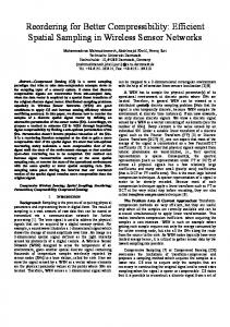
OPTIMAL CONTROL BASED DRIVER MODEL According to Donges [4] human vehicular control can be separated into guidance and stabilization. Accordingly, a two-level driver model is suggested consisting of an anticipation level, where nominal trajectories for vehicle guidance are selected, and a stabilization level, where suitable control actions for adhering to the reference input variables are implemented. In the two-level driver model developed in the following, nominal trajectories for the path and the speed profile of the vehicle are determined by optimal control methods. This approach is motivated by the optimal control model of Baron, Kleinman and Levison [1] for the stabilization level. Accordingly, a “well-motivated, welltrained human operator behaves in a near-optimal manner subject to his inherent limitations and constraints, and his control task.” While common models for the driver anticipation level select the road center line and the maximum permissible vehicle speed as trivial reference variables, we formulate the driving task as a parametric optimal control problem. To depict the driver’s motivation, a combination of suitable optimality criteria, such as maximum traveled distance and minimum mean-square values of the vehicle’s deviation from the road center line and the lateral acceleration, is used. In this regard, the current work extends the driver model of Ehmann et al. [5, 17] for racing applications where time-optimal set variables are computed. The optimal control approach promises an easily parameterizable, synthetic driver model which is suitable to investigate the objective vehicle handling properties in the computer over a broad range of drivers, maneuvers, tracks and vehicles. On the stabilization level, a non-linear position control algorithm serves to guide the vehicle precisely along the prescribed trajectories for path and speed profile. Some controller parameters, such as preview, controller gain and steering delay, may be adjusted to represent human properties in vehicle guidance [8]. As compared to classic driver models from linear control theory, this approach provides vehicular control independent of the respective driving maneuver and offers a small number of meaningful driver parameters. For a detailed discussion of other driver controllers we refer to [2]. ANTICIPATION LEVEL The computation of nominal path and speed trajectories for vehicle guidance requires a vehicle dynamics model which can be treated with optimal control methods. Suitable for this application is the single track model [11] shown in Fig. 3. The latter is a planar vehicle model where front and rear wheels are condensed to one single wheel each and the center of gravity is situated on road height. Vertical dynamics, pitch and roll motions as well as displacements of the wheels relative to the vehicle body are neglected. αf

lf

δf lr

β

Fy,f

ψ Fx,f

αr

Fx,r Fy,r

Figure 3: Single track model [11].

By means of reasonable simplifications the dynamics of the single track model can be summarized by the set of ordinary differential equations β& = −ω z +

ω& z =

1 Iz

v& =

1 m

1 mv

(F

y,r

(( F + F (F β + F y, f

y ,r

− Fx,r β + Fy , f + Fx , f (δ f − β ) )

x, f

x ,r

)δ f l f − Fy ,r l r ) − Fy , f (δ f − β ) + Fx , f

)

ψ& = ω z X& = v cos(ψ + β ) Y& = v sin(ψ + β ) δ& = ω . δ

Here, β denotes the side slip angle of the vehicle; ψ and ωz are the yaw angle and the yaw rate respectively. v is the velocity, and X and Y denote the position of the vehicle center of gravity in inertial coordinates. The steering wheel angle δ is treated as a separate model state with the steering velocity ωδ as derivative. With Fx,f and Fx,r we denote the traction and braking forces at the front and rear axle. With regard to the feasibility of the optimal control problem the respective lateral tire forces Fy,f and Fy,r are represented as linear functions of the tire side slip angles αf and αr :

l f ωz   − β  Fy , f = c f α f ≅ c f  δ f − v   l ω  Fy , r = c r α r ≅ c r  r z − β  .  v  In practice, this approximation is obviously not correct, since the maximum tire forces are bounded and skidding occurs for large values of the side slip angles. The validity of the single track model described here is therefore limited to normal vehicle operation with lateral accelerations of 5 m/s2 and less. Several optimality criteria which are eligible to depict the driver’s motivation, such as maximum traveled distance or minimum steering effort, are investigated in [2]. For the study in this paper, additional state equations 2 ∆& = (Y − µ ( X ) ) & = 12 (F + F Φ m

y ,r

y, f

)

2

are introduced which determine the mean-square deviation of the vehicle from the road center line (X) and the quadratic mean of the lateral acceleration respectively. For the classification of different driver types the parametric optimality criterion

ϕ ( p) = p1 (X (0) − X (t f ) ) + p 2 ∆(t f ) + p3 Φ (t f ) is selected which consists of partial criteria for the maximum traveled distance, the minimum accumulated deviation from the lane center and the minimum mean-square lateral acceleration. To guarantee equal weighting of the single objectives, suitable scaling factors must be included [2]. State constraints for the optimal control problem are given by two nonlinear inequalities which consider the limitations of the road track. Depending on the half vehicle width b/2, the constraints on the trajectory of the vehicle center of gravity result in g1 ( X , Y ) = q1 ( X ) − (Y + b2 ) ≥ 0 g 2 ( X , Y ) = (Y − b2 ) − q 2 ( X ) ≥ 0

where q1 and q2 denote the left and right borders of the driving lane respectively. In addition, control constraints − ω max ≤ ωδ (t ) ≤ ω max bounding the maximum steering motions due to physical limitations of the driver as well as box constraints on the traction and braking forces Fx,f, Fx,r are included. For the solution of the optimal control problem the direct collocation method DIRCOL [19] is used which enables low time requirements, since the integration of the dynamical system and the solution of the optimal control problem is carried out simultaneously. In this numerical algorithm, approximations for the problem quantities are computed on a discretization grid which is automatically refined during the iterations. The state variables x = (β, ωz, v, ψ, X, Y, δ) are discretized by piecewise cubic polynomials k

 t − t j −1   , t j −1 < t ≤ t j , j = 1,..., N , xˆ (t ) = ∑ c  t −t  k =0 j −1   j 3

k j

where suitable polynomial coefficients cjk are selected, such that the equations of motions are automatically fulfilled at the grid points tj of the discretization (collocation at Lobatto points). The control variables u = (ωδ,, Fx,f, Fx,r) are approximated by piecewise linear polynomials

 t − t j −1   (u − u j −1 ), t j −1 < t ≤ t j , uˆ (t ) = u j −1 +  t −t  j j −1   j with uj denoting their values at the grid points [18]. According to this discretization, the above optimal control problem is transcribed to a nonlinearly constrained large-scale optimization problem. The unknowns of this problem are the supporting values cj0 and uj at the grid points tj. The optimality criterion is given by a discretized version of ϕ(p). Nonlinear equality constraints arise from the equations of motion which are prescribed at the center points tj-1/2 + tj/2 of the discretization and, if applicable, from additional boundary conditions at the ends of the time interval. Moreover, nonlinear inequality constraints are present due to the road limitations enforced at all grid points. For the solution of the optimization problem, a suitable numerical algorithm is required which is able to consider the nonlinear constraints explicitly. Therefore, the sequential quadratic programming method SNOPT [6] is employed which exploits the sparse problem structure. In [2] also the inverse optimal control problem, i.e. estimating parameters of the optimality criterion ϕ(p) according to given reference data, is investigated. This requires the iterative solution of the above optimization problem in the context of standard parameter estimation techniques. The goal of this approach is to find optimal control parameters corresponding to certain clusters of drivers and enable the simulation of typical driver types. STABILIZATION LEVEL A large number of control algorithms is known in the literature which try to depict human vehicular control on the stabilization level. Most of these models have linear transfer behavior which basically constitutes a driver model being linearized about one special operating point [2, 9]. In practice, however, changing concentration, thresholds in perception and variable motivation of the driver lead to nonlinear or even discontinuous driving behavior. Thus, it is convenient to use a nonlinear control algorithm that is not tuned to one single driving situation. To model the control activities of the driver, we make use of the position controller veDYNA Driver [14] which is based on the concept of nonlinear system decoupling and control [10]. Input quantity for the controller is a set point for the nominal vehicle position which is basically determined by the nominal path and speed profiles.

The computation of the nonlinear position control relies on simplifications of the above single track model. For this purpose, the influence of the tire side forces Fy,f and Fy,r on the vehicle speed is neglected, and only traction and braking forces at the rear wheels are considered; yet, it should be noted that also front and all wheel drive can be implemented. Instead of the steering wheel angle δ the lateral force Fy,f at the front tire is used as second control variable besides Fx,r . According to [10], the set values of the position controller are obtained from F y , f = − Fy ,r + m [( β cos(ψ + β ) − sin(ψ + β )) a X ,des + ( β sin(ψ + β ) + cos(ψ + β )) aY , des ]

and Fx ,r = m [cos(ψ + β ) a X , des + sin(ψ + β ) aY ,des ] .

Here, aX,des and aY,des denote the desired accelerations of the vehicle which include the current deviations from the nominal position and velocity vector as well as stability parameters of the control. For actuating the steering wheel, the accelerator and the brake pedal of the vehicle, inverse characteristics of the tire forces and the engine as well as internal vehicle limitations are considered.

DOUBLE LANE CHANGE MANEUVER The expediency of the proposed driver model is investigated for a standard vehicle dynamics maneuver, i.e. the double lane change according to ISO 3888 [7]. In this maneuver, the vehicle path is constrained by three laterally displaced driving lanes of increasing width. For the following considerations, we confine ourselves to the constant maneuver speed of 80 km/h [7]. Therefore, it is sufficient to examine the vehicle trajectories for the eligible optimization criteria. For the driving tests from the next section a 1985 Ford Scorpio with measurement equipment was used. The parameters for the single track model were chosen accordingly. The same holds for the coefficients of the full vehicle model in veDYNA which is used as reference for realistic vehicle behavior and to determine the usability of the nominal vehicle paths computed from the optimal control problem. We first investigate the three basic optimality criteria which are part of the parametric cost functional for the driver’s motivation: MAXIMUM TRAVELED DISTANCE Racy driving style can be characterized by minimum driving time for a given course or by maximum traveled distance for fixed time. In the current lane change maneuver, however, variations in the traveled distance are limited due to the constant vehicle speed.

Figure 4: Comparison between nominal ( – – ) and full vehicle (  ) path for maximum traveled distance.

Figure 4 shows the vehicle trajectory for maximum traveled distance of the single track model (dashed line). The optimal vehicle path lies next to the inner bends of the driving lanes. Besides small deviations during the first lane change, the path controller in veDYNA is able to follow the nominal course rather accurately (solid line). Also the prescribed vehicle speed is observed very well. This is rather remarkable, since this maneuver effectuates maximum lateral accelerations of about 8 m/s2 which are outside the valid range of the single track model. Equally good correspondence between both vehicle models for this maneuver is reported by Ehmann et al. [17]. MINIMUM DEVIATION FROM THE LANE CENTER With regard to driving safety it is very import to stay in the current lane and avoid uncontrolled encounters with the traffic on other lanes and the environment of the road. A suitable criterion for the quality of lane keeping is to minimize the quadratic deviation from the lane center. This objective yields the nominal vehicle path depicted in Fig. 5 (dashed line). Due to the demanding steering task large steering movements and lateral accelerations are implemented. The comparison with the result of the full vehicle dynamics simulation (solid line) marks the differences between both models. In contrast to the single track model where arbitrarily large lateral forces can be obtained due to the linear tire characteristics, the wheel grip of the full vehicle model is limited and the nominal vehicle path cannot be traced exactly. A noticeable time delay occurs between both trajectories specifically during the lane changes and in the second lane. Closer inspection of the vehicle state variables reveals skidding in the second and third lane as well as corresponding cuts in the vehicle speed.

Figure 5: Comparison between nominal ( – – ) and full vehicle (  ) path for minimum deviation from the lane center. MINIMUM QUADRATIC LATERAL ACCELERATION Driving comfort is characterized by small inertial forces exerted on the passengers. Due to the plane vehicle model and the constant vehicle speed of the investigated maneuver, vertical and longitudinal accelerations cannot be considered in the optimal control problem. We are therefore restricted to the lateral vehicle motions. The criterion for minimum mean-square lateral acceleration yields the trajectory shown in Fig. 6 (dashed line). Similar trajectories are obtained when minimizing the quadratic mean values of slip angle, steering wheel angle and steering velocity [2]. A smooth, wavelike path characteristic is obtained which can be implemented with few steering effort.

Figure 6: Comparison between nominal ( – – ) and full vehicle (  ) path for minimum quadratic lateral acceleration. Accordingly, the simulation with veDYNA (solid line) results in good agreement between the state variables of both vehicle models. The dynamics of the entire driving maneuver lies inside the valid range of the reduced optimal control vehicle model; the lateral acceleration is limited by 3.5 m/s2. SUMMARY Three optimality criteria were presented which yield significantly distinct vehicle trajectories and, as a consequence, substantially distinct vehicle dynamics. The combination of these criteria is suitable to characterize various driving strategies for the double lane change maneuver. A video which visualizes the different vehicle and driver performances is available from [13]. When following the nominal vehicle paths with the full car model in veDYNA, rather good agreement between the prescribed and the implemented trajectories is obtained. Even for demanding driving maneuvers and vehicle dynamics outside the valid range of the single track model, i.e. specifically for the second optimality criterion, the nonlinear path controller on the stabilization level of the driver model shows very good quality in path following. The optimal solutions of the single track model are therefore feasible as input reference values for the vehicle dynamics simulation.

VARIATION OF THE DRIVER MODEL PARAMETERS With regard to implementing a wide range of driving strategies for virtual test drives, we carry out a systematic variation of the parameters of the optimality criterion ϕ(p). Due to lack of measurement data from less restrictive maneuvers, again the double lane change with a constant speed of 80 km/h is investigated.

Figure 7: Nominal trajectories for varied weighting parameters in the driver’s optimality criterion.

For the computation of nominal trajectories we vary the weighting parameters p1 and p2 of the criteria for maximum traveled distance and minimum deviation from the lane center between 0.2 and 5.0; the objective for minimum mean-square lateral acceleration is included with weights p3 between 0.05 and 20.0. The resulting full factorial design yields the band of trajectories depicted in Fig. 7. Despite the predetermined driving maneuver, we obtain a wide range of eligible vehicle paths for accomplishing the double lane change. For the comparison with real driving behavior, reference data from a number of average drivers between 21 and 58 years and heterogeneous driving experience was used. This data was obtained from former driving tests conducted at the Chair of Automotive Engineering at TU Darmstadt. Since the vehicle trajectory, which we use for the distinction of different driver types, was not recorded, only straightforward measurable vehicle states, such as the vehicle speed and some angular variables, were available for comparison. Accordingly, we compare the measured roll and steering wheel angles with the envelopes of the corresponding vehicle states when following the above nominal trajectories with the full vehicle dynamics model in veDYNA. The actual longitudinal speeds which were implemented in the tests deviated from the constant nominal speed and therefore required a synchronization of the state variables to the full maneuver length.

Figure 8: Comparison between measured roll angles (left) and steering wheel angles (right) and results from full vehicle dynamics simulation for varied weighting parameters in the driver’s optimality criterion. Figure 8 (left) shows a comparison between the roll angles obtained in the simulation and the driving tests. The variation of the weighting parameters yields good overlap of the measured data. Also the maximum amplitudes show good agreement, even though not the entire range of driving dynamics was implemented in the test drives. The characteristics from simulation show sharper outlines and thus better vehicle control which is due to the nonlinear path controller in veDYNA being superior to most human drivers. Similar results can be seen in Fig. 8 (right) where the respective steering wheel angles are compared. Again the state variables show basically good overlap. Not all extreme steering movements from the simulation were implemented in the tests; specifically, counter-steering due to skidding in the simulation (between 100 m and 110 m) did not occur. Also, in the second driving lane and at the end of the maneuver less precise steering movements as compared to the synthetic path controller are visible. Thus, by variably weighting the optimality criteria used for the computation of the nominal paths it is possible to cover a broad range of the vehicle dynamics spectrum. In addition, good overlap is examined with data from driving tests. We expect to achieve even bigger correspondence with the measurement data by also varying the parameters of the path controller on the stabilization level of the driver model, cf. [8].

CONCLUSIONS

In this paper, a driver model based on optimal control methods was presented. Nominal path and speed trajectories for vehicle guidance are obtained from the solution of an optimal control problem where a parametric optimality criterion is used to characterize different driving behavior. For the double lane change maneuver, eligible optimality criteria were examined and a variation of the weights in the parametric objective was carried out. A broad vehicle dynamics spectrum was implemented and essentially good overlap between the simulated and the observed driving behavior was achieved. Thus, the optimal control concept yields an efficient parametric driver model which can be employed to try out virtual prototypes and vehicle dynamics controllers for a wide range of different driver types and vehicles. Its feasibility for other driving maneuvers is to be examined. REFERENCES

1. S. Baron, D. L. Kleinman, W. H. Levison: An Optimal Control Model of Human Response, Part I+II, Automatica, 6, 1970, pp. 357-383. 2. T. Butz: Optimaltheoretische Modellierung und Identifizierung von Fahrereigenschaften. PhD Thesis, TU Darmstadt, 2004. 3. T. Butz, M. Ehmann, T.-M. Wolter: A Realistic Road Model for Real-Time Vehicle Dynamics Simulation. SAE Paper 2004-01-1068, 2004. 4. E. Donges: Experimentelle Untersuchung und regelungstechnische Modellierung des Lenkverhaltens von Kraftfahrern bei simulierter Straßenfahrt, PhD Thesis, TH Darmstadt, 1977. 5. M. Ehmann: A Real-Time Driver Model: Optimal Control, Guidance and Stabilization, PhD Thesis, TU Darmstadt, in preparation. 6. P. E. Gill, W. Murray, M. A. Saunders: SNOPT: An SQP algorithm for large-scale constrained optimization, SIAM Journal on Optimization, 12, 2002, pp. 979-1006. 7. International Organization for Standardization: ISO 3888-1: Passenger cars – Test track for a severe lanechange manoeuvre – Part 1: Double lane-change, Geneva, 1999. 8. M. Irmscher, M. Ehmann: Driver Classification Using veDYNA Advanced Driver. SAE Paper 2004-010451, 2004. 9. T. Jürgensohn: Hybride Fahrermodelle, ZMMS Spektrum Band 4, Pro Universitate Verlag, Sinzheim, 1997. 10. R. Mayr: Verfahren zur Bahnfolgeregelung für ein automatisch geführtes Fahrzeug, PhD Thesis, University Dortmund, 1991. 11. P. Rieckert, T. E. Schunck: Zur Fahrmechanik des gummibereiften Kraftfahrzeugs}, Ingenieur Archiv, 11, 1940, pp. 210-224. 12. G. Rill: Simulation von Kraftfahrzeugen, Vieweg, Braunschweig, 1994. 13. Simulation and Systems Optimization Group: Videos, World Wide Web, http://www.sim.informatik.tudarmstadt.de/videos/kfz3/. 14. TESIS DYNAware: veDYNA Driver Manual, 2002-2004. 15. TESIS DYNAware: veDYNA User Manual, 1996-2004. 16. M. Vögel: Fahrbahnmodellierung und Kursregelung für ein echtzeitfähiges Fahrdynamikprogramm, Diploma Thesis, TU München, 1997. 17. M. Vögel, O. von Stryk, R. Bulirsch, T.-M. Wolter, C. Chucholowski: An optimal control approach to realtime vehicle guidance. In: W. Jäger, H.-J. Krebs (eds.): Mathematics – Key Technology for the Future, Springer Verlag, Berlin, Heidelberg, 2003, pp. 84-102. 18. O. von Stryk: Numerische Lösung optimaler Steuerungsprobleme: Diskretisierung, Parameter-optimierung und Berechnung der adjungierten Variablen, Fortschritt-Berichte VDI,Reihe 8, Nr. 441, VDI-Verlag, Düsseldorf, 1995. 19. O. von Stryk: User's Guide for DIRCOL Version 2.1: A direct collocation method for the numerical solution of optimal control problems, Technical Report, rev. ed., Simulation and Systems Optimization Group, TU Darmstadt, 2001.