enhanced our ability to control engine operation utilizing ... development processes, engine calibration maps are ..... predetermined optimization criterion.
2008-01-1367
Optimal Engine Calibration for Individual Driving Styles Andreas A. Malikopoulos, Dennis N. Assanis, and Panos Y. Papalambros Automotive Research Center, The University of Michigan
Copyright © 2008 SAE International
only partially indicative of actual engine operation in a vehicle. The increasing sophistication of ECUs requires new technologies and methods in the design and development process.
ABSTRACT Increasing functionality of electronic control units has enhanced our ability to control engine operation utilizing calibration static maps that provide the values of several controllable variables. State-of-the-art simulation-based calibration methods permit the development of these maps with respect to extensive steady-state and limited transient operation of particular driving cycles. However, each individual driving style is different and rarely meets those test conditions. An alternative approach was recently implemented that considers the derivation of these maps while the engine is running the vehicle. In this approach, a self-learning controller selects in real time the optimum values of the controllable variables for the sequences of engine operating point transitions, corresponding to the driver’s driving style. This paper presents a quantitative assessment of the benefits in fuel economy and emissions, derived from employing a self-learning controller for optimal injection timing in a diesel engine. The engine is simulated over transient operation in response of a hypothetical driver’s driving style.
Advancements in computing technology have enabled simulation-based methods such as Hardware in the Loop (HiL) and Software in the Loop (SiL) test systems [6, 7]. HiL systems have been widely utilized as powerful methods for implementing engine calibration maps. These systems involve a real-time simulation engine model and a vehicle system connected to the ECU hardware. HiL systems allow the ECU development through simulation of powertrain components and vehicle system. SiL systems are more recent approaches, in which the engine model is integrated with the ECU software, and run on a computer [8]. SiL allows selective tests of single calibration tasks and separate modules of the ECU early in development. An essential requirement of HiL and SiL systems is the availability of an engine model capable of generating physical and consistent outputs of a combustion engine based on actual inputs. HiL and SiL systems aim to provide automated software tools for generating and validating calibration maps during the ECU development process. Further simulation-based methods for deriving these maps at steady-state engine operation have been extensively reported in the literature [9-12]. These efforts have been valuable in understanding steady-state operation, and optimizing fuel economy and emissions in recent years [13]. Transient engine operation, however, constitutes the largest segment in actual engine operation compared to the steady-state one [14]. Fuel consumption and emissions during transient operation are extremely complicated, vary significantly with each particular driving cycle [15, 16], and are highly dependent upon the calibration maps employed by the engine’s ECU [16, 17]. Research efforts in addressing transient operation have focused on simulation-based methods to derive calibration maps for transients of
INTRODUCTION Increasing demand for greater fuel economy and better performance, in conjunction with stringent emission legislation, has enhanced the functional range of electronic control units (ECUs). Current ECUs perform a variety of control tasks using engine calibration static maps that provide the values of several controllable variables. These values are referenced by actuators to maintain optimal engine operation. In traditional ECU development processes, engine calibration maps are generated experimentally by extensive steady-state engine operation and step function changes of engine speed and load [1-4]. This is usually accompanied by simple transient operation limited by dynamometer capabilities and simulation technologies [5]. However, steady-state and simple transient engine operation is 1
particular driving cycles. Burk et al. [18] presented the necessary procedures required to utilize co-simulation techniques with regard to predicting engine drive cycle performance for a typical vehicle. Jacquelin et al. [19] utilized analytical tools to run the FTP-75 driving cycle through pre-computed engine performance maps, depending on engine speed, load, intake and exhaust cam centerline positions. Atkinson et al. [20] implemented a dynamic system to provide optimal calibration for transient engine operation of particular driving cycles. These methods utilize engine models sufficiently accurate to portray fuel economy and feedgas emissions during transient engine operation. However, identifying all possible transients, and thus deriving optimal values of the controllable variables through calibration maps for those cases a priori, is infeasible.
identification and stochastic control problem is described. A study is performed on a four-cylinder, 1.9L turbocharged diesel engine to quantify the efficiency of this approach in deriving the optimal injection timing. Following the summary of our findings, conclusions are drawn in the last section.
MODELING ENGINE OPERATION AS A CONTROLLED STOCHASTIC PROCESS Engines are streamlined syntheses of complex physical processes determining a convoluted dynamic system. They are operated with reference to engine operating points and the values of various engine controllable variables. At each operating point, these values highly influence engine performance indices, e.g., fuel economy, emissions, engine performance. This influence becomes more prominent at engine operating point transitions designated partly by the driver’s driving style and partly by the engine’s controllable variables. Consequently, the engine is a system whose behavior is not completely foreseeable, and its future evolution (operating point transitions) depends on the driver’s driving style. In this context, the engine is treated as a stochastic system and the engine operating points are considered controlled random variables. This approach enables a stochastic quantification of the uncertainty regarding the future operating point transitions associated with the driver.
To address these issues, an alternative approach has been implemented that makes the engine of a vehicle an autonomous intelligent system capable of learning the values of various controllable variables in real time while the driver drives the vehicle [21]. Through this approach, engine calibration is optimized with respect to both steady-state and transient operation designated by the driver’s driving style. The engine is treated as a controlled stochastic system and engine calibration is formulated as a system identification and stochastic control problem. A real-time computational learning model has been implemented, suitable for solution of the state estimation and system identification sub-problem [22]. The model allows engine realization based on gradually enhanced knowledge of engine response as it transitions from one operating point to another. A lookahead control algorithm has been developed that solves the stochastic control problem by utilizing accumulated data acquired over the learning process of the computational model. The enhancement of the problem’s dimensionality, when more than one controllable variable is considered, was addressed by a decentralized learning control scheme [23]. This scheme draws from multi-agent learning research in a range of areas including reinforcement learning, and game theory to coordinate optimal behavior among the various controllable variables. The engine was modeled as a cooperative multi-agent system, in which the subsystems, i.e., controllable variables, were treated as autonomous intelligent agents who strive interactively and jointly to optimize engine performance criteria, e.g., fuel economy, emissions, etc.
The problem of deriving the values of the controllable variables for engine operating point transitions is compromised of two major sub-problems. The first concerns exploitation of the information acquired from the engine operation to identify its behavior, that is, how an engine representation can be built by observing engine operating point transitions. In control theory, this is addressed as a state estimation and system identification problem. The second concerns assessing the engine output with respect to alternative values of the controllable variables (control policies), and selecting those that optimize specified engine performance indices. This forms a stochastic control problem. In this context, the engine is treated as a controlled stochastic system and engine calibration is formulated as a sequential decision-making problem under uncertainty. The objective of the solution to this problem is to compute the values of the controllable variables for each engine operating point transition that optimize engine performance indices. These values are selected at points of time referred to as decision epochs (or stages), where the time domain can be either discrete or continuous. In our case, discrete time is employed because of the discreteness in the values of the variables (control actions). The engine output is sampled at the decision epochs. The stochastic system model aims to provide the mathematical framework for analysis of the sequential decision-making problem in this stochastic environment.
This paper reports work in applying the aforementioned approach to derive in real time the optimal injection timing in a diesel engine over transient engine operation as a result of a hypothetical driver’s driving style. This work permits a quantitative assessment of the improvement of fuel economy and emissions. The remainder of the paper proceeds as follows. The next section presents modeling of engine operation as a controlled stochastic process. Then, the formulation of the engine calibration problem as an engine 2
the random variables s0 , s1 ,..., v0 , v1 ,... , and thus, is also a random variable. Similarly, the sequence of the values of controllable variables ak = µ ( sk ) , {ak , k ≥ 0} , constitutes a stochastic process.
STOCHASTIC SYSTEM MODEL The stochastic system model [24, 25], illustrated in Figure 1, has two principal features: (a) an underlying dynamic system (engine); and (b) an evaluation function (engine output). The dynamic system is denoted by sk +1 = f k ( sk , α k , wk ), k = 0,1,..., M − 1
(1)
yk = hk ( sk , vk ),
(2)
Definition 1. The random variables s0 , w0 , w1 ,..., v0 , v1 ,..., are the basic random variables, since the sequences {sk , k ≥ 0} and {ak , k ≥ 0} are constructed from them. We explore whether the conditional probability distribution of sk +1 given sk and ak is independent of previous values of states and control actions. Suppose the control policy π = {µ0 , µ1 ,..., µ M −1} is employed. The
where sk represents the state (engine operating point), which belongs to the finite engine operating space S , and ak represents the control action (values of the controllable variables) at time k. These values belong to some feasible action set A( sk ) , which is a subset of the control space A . The sequence {wk , k ≥ 0} is an unknown disturbance representing the driver while commanding the engine through the accelerator pedal. This sequence represents the driver’s driving style, and thus, it is treated as a stochastic process with an unknown probability distribution; yk is the engine output, and vk is the measurement sensor error or noise. The sequence {vk , k ≥ 0} is treated as a stochastic process with unknown probability distribution.
corresponding
αk
ykπ = hk ( skπ , vk ).
(4)
akπ = µ ( skπ )
(5)
Psπk +1 | sk , ak ( sk +1 | sk , ak ) = Pwπk | sk , ak ( wk | sk , ak ),
(6)
(7)
The interpretation of Eq. (7) is that the conditional probability of reaching the engine operating point sk +1 at time k + 1 given sk and ak is equal to the probability of being at the pedal position wk at time k. Suppose that the previous values of the random variables sm and am , m ≤ k − 1 are known. The conditional distribution of sk +1 given these values will be
vk Engine Output hk
(3)
For any operating point sk +1 , at time k + 1 , and from Eq. (3), we have
Sensors
sk
skπ+1 = f k ( skπ , akπ , wk ), s0π = s0 ,
Psπk +1 | sk , ak (⋅ | sk , ak ).
The state sk depends upon the input sequence a0 , a1 ,..., aM −1 as well as the random variables w0 , w1 ,..., wk , Eq. (1). Consequently, sk is a random variable; the engine output yk = hk ( sk , vk ) is a function of
Engine fk
{skπ , k ≥ 0) ,
Suppose further that the values realized by the random variables sk and ak are known. These values are insufficient to determine the value of sk +1 since wk is not known. The value of sk +1 is statistically determined by the conditional distribution of sk +1 given sk and ak , namely
We seek a finite sequence of functions π = {µ0 , µ1 ,..., µ M −1}, defined as a control policy, which minimizes the total cost, e.g., fuel consumption, emissions, etc, over M decision epochs. The functions µ k specify the control ak = µ ( sk ) that will be chosen when at the kth decision epoch.
wk
processes
{ ykπ , k ≥ 0) , and {akπ , k ≥ 0) , are defined by
Assumption 1. The engine output can be fully observed.
Driver
stochastic
yk
Psπk +1 | sk , ak ( sk +1 | sk ,..., s0 , ak ,..., a0 ) = = Pwπk |sk , ak ( wk | sk ,..., s0 , ak ,..., a0 ).
Self-Learning Controller πk
(8)
The conditional probability distribution of sk +1 given sk and ak can be independent of the previous values of states and control actions, if it is guaranteed that for
Figure 1. The stochastic system model adapted for the engine calibration problem. 3
every control policy π , wk is independent of the random variables sm and am , m ≤ k − 1 . Kumar and Varaiya [24] proved that this property is imposed under the following assumption.
Rk (sk+1| sk, αk)
…
Assumption 2. The basic random variables s0 , w0 , w1 ,..., v0 , v1 ,..., are all independent. This is, indeed, true in reality since the initial operating point s0 as well as the sequence of accelerator pedal positions {wk , k ≥ 0} and the sequence of sensor errors {vk , k ≥ 0} are not related. Assumption 2 imposes a condition directly on the basic random variables which eventually yields that the engine operating point sk +1 depends only on sk and ak . Moreover, the conditional probability distributions do not depend on the control policy π , and thus, the subscript π can be dropped Psk +1 | sk , ak ( sk +1 | sk ,..., s0 , ak ,..., a0 ) = Psk +1 | sk , ak ( sk +1 | sk , ak ).
Rk+1 (sk+2| sk+1, αk+1)
… sk
sk+1
sk+2
Decision Epoch k
Decision Epoch k+1
Decision Epoch k+2
Figure 2. Sequential decision-making adapted in the engine calibration problem.
OPTIMALITY CRITERIA The solution to an MDP can be expressed as an admissible control policy so that a given performance criterion is optimized over all admissible policies Π. An admissible policy consists of a sequence of functions
(9)
π = {µ0 , µ1 ,..., µ M −1},
A stochastic process {sk , k ≥ 0} satisfying the condition of Eq. (9) is called a Markov Process and the aforementioned condition is the Markov property.
(10)
where µ k maps states sk into actions α k = µ k ( sk ) and is such that µk ( sk ) ∈ A( sk ), ∀sk ∈ S . A Markov policy π determines the probability distribution of state process {sk , k ≥ 0} and the control process {ak , k ≥ 0} . Different policies will lead to different probability distributions. In optimal control problems, the objective is to derive the optimal control policy that minimizes the accumulated cost incurred at each state transition per decision epoch. If a policy π is fixed, the cost incurred by π , when the process starts from an initial state s0 and up to the time horizon M, is
Definition 2 [26]. A Markov process is a random process {sk , k ≥ 0} with the property that given the values of the process from time zero up through the current time, the conditional probability of the value of the process at any future time depends only on its value at the current time. That is, the future and past are conditionally independent given the present. A large class of sequential decision-making problems under uncertainty can be modeled as a Markov Decision Process (MDP). MDP [27] provides the mathematical framework for modeling decision making in situations where outcomes are partly random and partly under the control of the decision maker. In this framework, the decision maker (controller) is faced with the problem of influencing engine behavior as it evolves over time, by selecting control actions (values of the controllable variables). The objective of the decision maker is to select these values of the controllable variables that make the engine perform optimally with respect to some predetermined optimization criterion.
J π ( s0 ) =
M −1
∑ R (s k =0
k
k +1
= j | sk = i, ak ),
(11)
∀i, j ∈ S , ∀ak ∈ A( sk ).
The accumulated cost J π ( s0 ) is a random variable since sk and ak are random variables. Hence the expected accumulated cost of a Markov policy is given by J π ( s0 ) =
Consequently, at each decision epoch k, the engine operates at a given state sk designated partly by the driver wk −1 , and partly by the controllable variable ak −1 at time k-1. On that basis the self-learning controller selects a value ak . One decision epoch later, the engine transits to a new state sk +1 and the controller observes the engine output yk +1 = hk +1 ( sk +1 , vk +1 ) = Rk ( sk +1 | sk , ak ) associated with this state transition, as illustrated in Figure 2.
=
M −1
E { ∑ Rk ( sk +1 = j | sk = i, ak )} =
sk ∈S ak ∈ A ( sk ) k = 0
M −1
E { ∑ Rk ( sk +1 = j | sk = i, µk ( sk ))},
sk ∈S ak ∈ A ( sk ) k = 0
(12)
The expectation is with respect to the probability distribution of {sk , k ≥ 0} and {ak , k ≥ 0} determined by the Markov policy π . Consequently, the control policy 4
that minimizes Eq. (12) is defined as the optimal Markov policy π ∗ .
style and eventually learn its optimal calibration for this driving style. The longer the engine runs during a particular driving style, the better the engine’s specified performance indices will be. The main reason for this is the ability to capture the stationary distribution of the engine operating point transitions associated with the driver’s driving style.
Dynamic programming (DP) has been widely employed as the principal method for computing global optimal policies in sequential decision-making problems under uncertainty. Algorithms, such as value iteration, policy iteration, and linear programming, have been extensively utilized in solving deterministic and stochastic optimal control problems, Markov and semi-Markov decision problems, and min-max control problems. However, the computational complexity of these algorithms in some occasions may be prohibitive and can grow intractably with the size of the problem and its related data, referred to as the DP “curse of dimensionality” [28]. In addition, DP algorithms require the realization of the conditional probabilities of state transitions and the associated costs, implying a priori knowledge of the engine realization. However, even if the transition probabilities are known, the problem of analytic computation might be too hard, and one might seek an approximation method.
SELF-LEARNING INJECTION TIMING IN A DIESEL ENGINE Both identification of engine operation and stochastic control problems were solved by conducting real-time simulation of a four-cylinder, 1.9L turbocharged diesel engine. The software package enDYNA Themos CRTD by TESIS [29] suitable for real-time simulation of diesel engines was employed. The software utilizes thermodynamic models of the gas path and is well suited for testing and development of ECUs. It can simulate the longitudinal vehicle dynamics with a highly variable drive train including the modules of starter, brake, clutch, converter, and transmission. In the driving mode the engine is operated by means of the usual vehicle control elements just as a driver would do. The driver model is designed to operate the vehicle at given speed profiles (driving cycles). It actuates the starter, accelerator, clutch and brake pedals according to the profile specification, and also shifts gears.
ENGINE IDENTIFICATION AND STOCHASTIC CONTROL The realization of the conditional probability distribution of the engine operating point transitions Eq. (9) constitutes the state estimation and engine identification problem. It has been shown that this realization is conditional depended on the driver’s driving style expressed by means of the sequences of the pedal position {wk , k ≥ 0} , Eq. (8). Consequently, to derive the values of the controllable variables suited for the driver’s driving style, real-time implementation is necessary, and thus, we seek for lookahead control policies.
The goal of the study was to evaluate the efficiency of the self-learning controller in identifying transient engine operation, and deriving the optimal control policy (main injection timing) to maximize engine torque. A single vehicle speed profile (driving cycle), shown in Figure 3, including an acceleration and deceleration segment designated by a hypothetical driver, was selected. The model was run repeatedly over the same speed profile, to represent a situation in which the driver desires a particular vehicle’s speed profile deemed characteristic of his/her driving style. The belief implicit here is that if the controller can successfully capture this profile, then it will also be able to capture engine realization designated by a driver in long term.
For the state estimation and engine identification subproblem, a computational model suited for real-time sequential decision-making under uncertainty has been implemented [22]. The model consists of a state-space representation constructed through a learning mechanism which can be used simultaneously in solving the stochastic control problem. Furthermore, it utilizes an evaluation function suitable for lookahead control algorithms, and thus, for real-time implementation. The model allows decision making based on gradually enhanced knowledge of engine response as it transitions from one operating point to another, in conjunction with the values of the controllable variables selected at each operating point. While the engine interacts with the driver, the model learns the engine realization in terms of the Markov state transitions. To enable the engine to select the values of various controllable variables in real time, a lookahead control algorithm has been developed [21]. The algorithm solves the stochastic control sub-problem by utilizing accumulated data acquired over the learning process of the state-space representation. The combination of the state-space representation and control algorithm makes the engine progressively perceive the driver’s driving
The model with the baseline ECU incorporates a static calibration map for injection timing corresponding to steady-state operating points. Before initiating the first simulation, the model with the self-learning controller has no knowledge regarding the particular transient engine operation and injection timing associated with it. The controller has been regulated to select any values of injection timing between -2º and 18º before top dead center (BTDC). This is considered the feasible set of allowable values of injection timing and it can be assigned differently depending on the engine. The decision epochs are the discrete time steps in which the controller observes the engine output and selects the value of injection timing. The decision epoch can be assigned to be either constant or varying. In this example, the decision epoch is constant and equal to 5
the time step used by the ECU baseline calibration map to interpolate the static maps. 100
QUANTITAVE ASSEMENT OF BENEFITS IN FUEL CONSUMPTION AND EMISSIONS
90
Pedal Position [%]
After completing the exploration phase, the self-learning controller derived the values of injection timing, shown in Figure 4. The significant variation of injection timing is attributed to the engine behavior during the transient period before steady-state operation occurs. During this period, the maximum brake torque (MBT), and thus, brake-specific fuel consumption and emissions, are varied for the same engine operating point [21]. These values, corresponding to a particular operating point, highly depend on the previous operating points from which they have been arrived. Consequently, start of injection at steady-state operating points is not optimal for the same points when transiting from different previous points.
50 40 30
0
0
5
10
15 Time [sec]
20
25
Figure 5. Pedal position rate.
3000
2500 Engine Speed [RPM]
Vehicle Velocity [mph]
60
10
20
15
10
5
Desired Speed Profile Model with Baseline ECU Model with Self-Learning Controller 0
5
10
15 Time [sec]
20
18
2000
1500
1000 Model with Baseline ECU Model with Self-Learning Controller
500
0
25
Figure 3. Desired speed profile.
0
5
10
15 Time [sec]
20
25
Figure 6. Engine speed.
Model with Baseline ECU Model with Self-Learning Controller
16 Injection Timing BTDC [deg]
70
20
25
0
Model with Baseline ECU Model with Self-Learning Controller
80
14 12 10 8 6 4 2 0 -2 0
5
10
15 Time [sec]
20
25
Figure 7. Engine operating point transitions.
Figure 4. Injection timing.
6
1.4
1
HC Concentration [%]
Injection Duration [ms]
0.025
Model with Baseline ECU Model with Self-Learning Controller
1.2
0.8 0.6 0.4
Model with Baseline ECU Model with Self-Learning Controller
0.02
0.015
0.01
0.005 0.2 0
0
5
10
15 Time [sec]
20
0
25
Figure 8. Injection duration.
x 10
7 Model with Baseline ECU Model with Self-Learning Controller
x 10
10
15 Time [sec]
20
25
-6
Model with Baseline ECU Model with Self-Learning Controller
6
2.5 PM Concentration [%]
Fuel Consumption [kg/sec]
5
Figure 11. HC concentration of emissions.
-3
3
0
2 1.5 1 0.5
5 4 3 2 1
0 0
5
10
15 Time [sec]
20
0
25
0
5
Figure 9. Fuel consumption.
15 Time [sec]
20
25
Figure 12. PM Concentration. x 10
0.06
10
-3
1.6
Model with Baseline ECU Model with Self-Learning Controller
Model with Baseline ECU Model with Self-Learning Controller
1.4 CO Concentration [%]
Mass Air Flow [kg/sec]
0.05 0.04 0.03 0.02
1.2 1 0.8 0.6 0.4
0.01
0.2
0 0
5
10
15 Time [sec]
20
0
25
Figure 10. Mass air flow into the cylinders.
0
5
10
15 Time [sec]
20
25
Figure 13. CO concentration of emissions.
7
Table 1 summarizes the quantitative assessment of the improvement of fuel consumption, and emissions, by employing the self-learning controller in ECU development.
1000 Exhaust Manifold Temperature [K]
900 800 700
Table 1: Quantification assessment of benefits with selflearning controller compared to baseline ECU.
600 500 400 300 200
Model with Baseline ECU Model with Self-Learning Controller
100 0
0
5
10
15 Time [sec]
20
Improvement [%]
Fuel consumption
8.4
NOx
7.7
HC
32.9
CO
5.0
PM
9.8
25
Figure 14. Exhaust manifold temperature.
x 10
Engine Performance Indices
-3
Model with Baseline ECU Model with Self-Learning Controller
1.6 1.4
SUMMARY AND CONCLUDING REMARKS
NOx Concentration [%]
1.2
We presented an approach for real-time engine calibration, treated as engine identification and stochastic control problems. A self-learning controller solves these two problems simultaneously. That is, while the driver drives the vehicle, the controller identifies engine realization as designated by the driver’s driving style. At the same time, the controller utilizes a lookahead algorithm to derive the values of the controllable variables for this realization. This approach permits real-time ECU development with respect to steady-state and transient engine operation resulting from a particular driving style.
1 0.8 0.6 0.4 0.2 0
0
5
10
15 Time [sec]
20
25
Figure 15. NOx concentration of emissions.
The case study presented a quantitative assessment of the improvement of fuel economy and emissions by employing this approach. The self-learning controller derived the optimal injection timing in a diesel engine over transient engine operation as a result of a hypothetical driver’s driving style. Future research should investigate the impact of different driver patterns on fuel consumption and emissions by utilizing statistical data of a diverse group of people. Drivability issues that may be raised in implementing this approach in a real vehicle should also be investigated.
The injection timing computed by the self-learning controller maximized engine torque during transient operation, and the desired speed profile was achieved requiring lower pedal position rates for the same engine speed, as illustrated in Figures 5 and 6. The implication is that injection timing altered the brake mean effective pressure (BMEP) for this range of engine speed, and engine operation was modified as shown in Figure 7. Lower pedal position rates required less injected fuel mass into the cylinders since injection duration was reduced (Figure 8), resulting in minimization of fuel consumption as illustrated in Figure 9. While the fuel mass injected into the cylinders is reduced, the mass air flow was kept almost constant (Figure 10) providing excess of air. These conditions degraded the formation of HC, CO and PM as illustrated in Figures 11-13. The injection timing of the baseline ECU provided higher emission temperatures in the exhaust manifold, shown in Figure 14, and consequently, NOx formation progressed much faster, as depicted in Figure 15.
ACKNOWLEDGMENTS This research was partially supported by the Automotive Research Center (ARC), a U.S. Army Center of Excellence in Modeling and Simulation of Ground Vehicles at the University of Michigan. The engine simulation package enDYNA Themos CRTD was provided by TESIS DYNAware GmbH. This support is gratefully acknowledged. The authors appreciate also valuable comments received by Dr. George Lavoie. 8
[12] Jankovic, M. and Magner, S., "Fuel Economy Optimization in Automotive Engines," Proceedings of the 2006 American Control Conference, Minneapolis, MN, USA, 2006. [13] Hagena, J. R., Filipi, Z. S., and Assanis, D. N., "Transient Diesel Emissions: Analysis of Engine Operation During a Tip-In," SAE 2006 World Congress, Detroit, Michigan, April 3-6, 2006, SAE 2006-01-1151. [14] Wijetunge, R. S., Brace, C. J., Hawley, J. G., Vaughan, N. D., Horroocks, R. W., and Bird, G. L., "Dynamic Behavior of a High-Speed, DirectInjection Diesel Engine," SAE Transactions-Journal of Engines, v. 108, 1999, SAE 1999-01-0829. [15] Clark, N. N., Gautam, M., Rapp, B. L., Lyons, D. W., Graboski, M. S., McCormick, R. L., Alleman, T. L., and National, P. N., "Diesel and CNG Transit Bus Emissions Characterization by Two Chassis Dynamometer Laboratories: Results and Issues," SAE Transactions-Journal of Fuels and Lubricants, v. 108, 1999, SAE 1999-01-1469. [16] Samulski, M. J. and Jackson, C. C., "Effects of Steady-State and Transient Operation on Exhaust Emissions from Nonroad and Highway Diesel Engines," SAE Transactions-Journal of Engines, v. 107, 1998, SAE 982044. [17] Green, R. M., "Measuring the Cylinder-to-Cylinder EGR Distribution in the Intake of a Diesel Engine During Transient Operation," SAE TransactionsJournal of Engines, v. 109, 2000, SAE 2000-012866. [18] Burk, R., Jacquelin, F., and Wakeman, R., "A Contribution to Predictive Engine Calibration Based on Vehicle Drive Cycle Performance," SAE 2003 World Congress, Detroit, Michigan, USA, March 36, 2003, SAE 2003-01-0225. [19] Jacquelin, F., Burk, R., and Wakeman, R. J., "Cam Phaser Actuation Rate Performance Impact on Fuel Consumption and NOx Emissions Over the FTP-75 Drive Cycle," SAE 2003 World Congress, Detroit, Michigan, USA, 2003, SAE 2003-01-0023. [20] Atkinson, C. and Mott, G., "Dynamic Model-Based Calibration Optimization: An Introduction and Application to Diesel Engines," SAE World Congress, Detroit, Michigan, April 11-14, 2005, SAE 2005-01-0026. [21] Malikopoulos, A. A., Papalambros, P. Y., and Assanis, D. N., "A Learning Algorithm for Optimal Internal Combustion Engine Calibration in Real Time," Proceedings of the ASME 2007 International Design Engineering Technical Conferences Computers and Information in Engineering Conference, Las Vegas, Nevada, September 4-7, 2007. [22] Malikopoulos, A. A., Papalambros, P. Y., and Assanis, D. N., "A State-Space Representation Model and Learning Algorithm for Real-Time Decision-Making Under Uncertainty," Proceedings of the 2007 ASME International Mechanical Engineering Congress and Exposition, Seattle, Washington, November 11-15, 2007.
REFERENCES [1] Roepke, K. and Fischer, M., "Efficient Layout and Calibration of Variable Valve Trains," SAE Transactions-Journal of Engines, v. 110, 2001, SAE 2001-01-0668. [2] Stuhler, H., Kruse, T., Stuber, A., Gschweitl, K., Piock, W., Pfluegl, H., and Lick, P., "Automated Model-Based GDI Engine Calibration Adaptive Online DoE Approach," SAE 2002 World Congress, Detroit, Michigan, March 3-7, 2002, SAE 2002-010708. [3] Brooks, T., Lumsden, G., and H.Blaxill, "Improving Base Engine Calibrations for Diesel Vehicles Through the Use of DoE and Optimization Techniques," Powertrain and Fluid Systems Conference and Exhibition, San Antonio, Texas, USA, September 24-27, 2005, SAE 2005-01-3833. [4] Knafl, A., Hagena, J. R., Filipi, Z. S., and Assanis, D. N., "Dual-Use Engine Calibration: Leveraging Modern Technologies to Improve PerformanceEmissions Tradeoff," SAE Word Congress, Detroit, Michigan, April 11-14, 2005, SAE 2005-01-1549. [5] Steiber, J., Trader, A., Reese, R., Bedard, M., Musial, M., and Treichel, B., "Development of an Engine Test Cell for Rapid Evaluation of Advanced Powertrain Technologies Using Model-Controlled Dynamometers," SAE Transactions-Journal of Passenger Cars- Electronics & Electrical Systems, v. 115, 2006, SAE 2006-01-1409. [6] Schuette, H. and Ploeger, M., "Hardware-in-theLoop Testing of Engine Control Units - A Technical Survey," SAE 2007 World Congress and Exhibition, Detroit, Michigan, April 16-19, 2007, SAE 2007-010500. [7] Philipp, O., Buhl, M., Diehl, S., Huber, M., Roehlich, S., and Thalhauser, J., "Engine ECU Function Development Using Software-in-the-Loop Methodology," SAE 2005 World Congress and Exhibition, Detroit, Michigan, 2005, SAE 2005-010049. [8] Caraceni, A., Cristofaro, F. D., Ferrana, F., and Scala, S., "Benefits of Using a Real-Time Engine Model During Engine ECU Development," SAE 2003 World Congress and Exhibition, March 3-6, 2003, SAE 2003-01-1049. [9] Guerrier, M. and Cawsey, P., "The Development of Model-Based Methodologies for Gasoline IC Engine Calibration," SAE Transactions-Journal of Engines, v. 113, 2004, SAE 2004-01-1466. [10] Rask, E. and Sellnau, M., "Simulation-Based Engine Calibration: Tools, Techniques, and Applications," SAE Transactions-Journal of Engines, v. 113, 2004, SAE 2004-01-1264. [11] Wu, B., Prucka, R. G., Filipi, Z. S., Kramer, D. M., and Ohl, G. L., "Cam-Phasing Optimization Using Artificial Neural Networks as Surrogate Models~Maximizing Torque Output," SAE Transactions-Journal of Engines, v. 114, 2005, SAE 2005-01-3757. 9
[26] Kemeny, J. G. and Snell, J. L., Finite Markov Chains, 1st edition, Springer, December 5, 1983. [27] Puterman, M. L., Markov Decision Processes: Discrete Stochastic Dynamic Programming, 2nd Rev. edition, Wiley-Interscience, 2005. [28] Gosavi, A., "Reinforcement Learning for Long-Run Average Cost," European Journal of Operational Research, vol. 155, pp. 654-74, 2004. [29] TESIS, .
[23] Malikopoulos, A. A., Assanis, D. N., and Papalambros, P. Y., "Real-Time, Self-Learning Optimization of Diesel Engine Calibration," Proceedings of the 2007 Fall Technical Conference of the ASME Internal Combustion Engine Division, Charleston, South Carolina, October 14-17, 2007. [24] Kumar, P. R. and Varaiya, P., Stochastic Systems, Prentice Hall, June 1986. [25] Bertsekas, D. P., Dynamic Programming and Optimal Control (Volumes 1 and 2), Athena Scientific, September 2001.
10