Title: Optimal Network Service Curves under Bandwidth-Delay Decoupling Author: Jens Schmitt Affiliation: Jens Schmitt Multimedia Communications (KOM), Department of Electronic Engineering & Information Technology, Darmstadt University of Technology, Germany, Merckstr. 25, 64283 Darmstadt, Germany Tel.: +49-6151-166163 Fax: +49-6151-166152
[email protected]
1
Optimal Network Service Curves under Bandwidth-Delay Decoupling Jens Schmitt
Abstract: Providing Quality of Service (QoS) guarantees to data flows in packet-switched networks like the Internet has been and still is an important research area. In particular, it is important to ensure strict (deterministic) guarantees for highly time-sensitive data flows. In this work, we derive optimal network service curves for deterministic service flows which are scheduled by bandwidth-delay decoupled service disciplines. Introduction: In future multi-service IP (Internet Protocol) networks, deterministic services which give strict guarantees on delay and loss characteristics are important, if those networks really want to take over the traffic served by specialized legacy networks. Certainly, deterministic services may not constitute the major part of the overall carried traffic, yet their expensive implementation makes them nevertheless attractive for optimization with respect to resource allocation. An important insight for the resource allocation optimization of deterministic services is that delay and bandwidth need to be decoupled to achieve efficient resource allocations. While in many approaches this decoupling has not been taken into account, e.g., the famous work by Parekh and Gallagher [1], more recent work has done so, see for example [2]. The latter proposes a bandwidth-delay decoupling scheduling scheme, which is based on non-linear scheduling discipline. In principle, they, like other approaches to decouple bandwidth and delay, propose piecewise linear service curves. Yet, none of these has dealt with an optimal choice of parameters of the piece-wise linear service curve for a given (regulated) input traffic flow. This is what we focus on here.
2
Network Calculus for Deterministic Services: The mathematics of deterministic services, commonly called network calculus, are originally based on the work of Cruz [Cru95] on arrival and service curves. While arrival curves describe the worst-case behavior of a source within given time intervals, service curves specify the minimal service that is provided by a queue service discipline. By combining these two concepts it is possible to derive deterministic guarantees on loss and delay under the worst-case scenario of a greedy source and a fully loaded server. A typical and often used arrival curve is the so-called TSpec(r,b,p,M) [3], defined by
a
TSpec
( t ) = M + pt t < T b + rt t ≥ T
,
(1)
where T = ( b – M ) ⁄ ( p – r ) may be considered as burst duration. The TSpec is essentially a double token bucket, where burstiness is accounted for by the first bucket characterized by peak rate p and maximum packet size M, and the long-term behavior is captured by the second token bucket characterized by average rate r and a bucket size b. A typical (linear) service curve for deterministic services [4] is
s
linear
+ t≤V , 0 (t) = R(t – V) = R(t – V) t > V
(2)
where V = C ⁄ R + D and R is the service rate assigned to a data flow by the respective queue service discipline, assuming that the stability condition R ≥ r holds. Here, the C and D terms represent the rate-dependent respectively rate-independent deviations of a packet-based scheduler from the perfect fluid model as introduced by [1]. These error terms are summed up along the data transmission path for each server/router during an advertisement phase. Applying network calculus we can compute delay bounds based on arrival and service curve:
3
d max = h ( a, s ) = sup s ≥ 0 ( inf { H: H ≥ 0 ∧ a ( t ) ≤ s ( t + H ) ) } )
(3)
For the TSpec as arrival curve and the linear service curve defined in (2) this results in
d max
( p – R) M + C T - + --------------- + D -------------------R R = M+C --------------- + D R
p≥R≥r (4) R≥p≥r
From the perspective of the receiver desiring a maximum queuing delay dmax, the service rate R that has to be reserved at the routers on the path from the sender follows directly: pT + M + C ------------------------------+T–D d R = max M+C ------------------- d max – D
d max ≤ d d max > d
M+C , where d = --------------- + D p
(5)
Bandwidth-Delay Decoupling of Service Curves: To use a linear service curve as done in the formulas above may lead to wasteful resource allocations, in particular, for “low bandwidth, short delay”-type of flows. For example consider a data flow with TSpec = (2000, 1000, 8000, 500) [in bytes resp. bytes/s]. Let us assume 5 hops (all with MTU = 9188 bytes and link speed c = 155 Mb/ s) all doing PGPS (Packetized General Processor Sharing) [1]. Then we have C = 5M = 7500 bytes and D = MTU/c = 2.371 ms. Let us further assume the receiver desires a maximum queueing delay of dmax = 100 ms. Then we obtain from the formulas given above that R = 30729 bytes/s ≈ 4p = 16r. That means in order to ensure a fairly strict delay bound the rate assignment of a flow is extremely over-provisioned in relation to its bandwidth requirements. The solution here is to decouple the bandwidth assignment from delay goals which can only be achieved by non-linear service curves. The most simple non-linear service curve that can achieve
4
bandwidth-delay decoupling is a continuous piece-wise linear service curve consisting of two linear segments, i.e., a service curve of the form R ( t – V )+ s (t ) = qt + f
t d : s ( t ) = R – r) rt + b 1 – --1- + rT (---------------–V R R
rT + b t < --------------- + V R rT + b t ≥ --------------- + VT R
b – rd max + RV R (t – V )+ t < ------------------------------------R–r opt d max ≤ d : s ( t ) = b – rd max + RV rt b rd t ≥ + – ------------------------------------max R–r This service curve, s
opt
pT + M + C with R = ------------------------------d max + T – D
M+C with R = --------------------d max – D
(8)
, is optimal in the sense that the inflection point I is “shifted” as far left as
possible without spending more resources on the short time-scales of the service curve than the linear service curve, s
linear
, and the simple non-linear service curve, s
simple
. This restriction on
the optimal service curve is reasonable since the short time-scales of service have to deal with satisfying delay bounds and are thus the rate resources most heavily contended for (especially if we deal with concave service curves as typically assumed for real-time services). Numerical Example: Reconsider the “low bandwidth, short delay”-type of flow taken as an example above already. For such a flow the different service curve assignments are shown in Figure 1. It is obvious that the linear service curve approach wastes a lot of bandwidth, the fact which led to the consideration of non-linear service curves. In comparison of the simple vs. the optimal non-linear service curve it can also be observed that the savings in terms of the shifting of the inflection point are considerable for this example: I is located about 65 ms earlier for the optimal than for the simple non-linear service curve. Summary: In this work we have derived explicit formulas for optimal service curves based on bandwidth-delay decoupling service disciplines. Furthermore, we have shown their potential
6
when compared to “intuitive / naive” choice of service curve parameters by a numerical example. Their full potential can be exploited especially in the case where “low bandwidth, short delay”type of flows are multiplexed with less delay-critical flows which can take advantage of the relative moderateness of the optimal service curves on longer time-scales. References: [1]
A. K. Parekh and R. G. Gallagher. A Generalized Processor Sharing Approach to Flow Control in Integrated Services Networks: The Single-Node Case. IEEE/ACM Transactions on Networking, 1(3):344–357, June 1993.
[2]
I. Stoica, H. Zhang, and T. S. E. Ng. Hierarchical Fair Service Curve Algorithm for LinkSharing, Real-Time and Priority Service. ACM Computer Communication Review, 27(4), October 1997. Proceedings of SIGCOMM’97 Conference.
[3]
J. Wroclawski. The Use of RSVP with IETF Integrated Services. Proposed Standard RFC 2210, September 1997.
[4]
S. Shenker, C. Partridge, and R. Guerin. Specification of Guaranteed Quality of Service. Proposed Standard RFC 2212, September 1997.
Figures: Figure 1: Different service curves for the given example flow.
7
14000
Rate (in bytes/s)
12000 10000
slinear
8000 6000
ssimple
4000 2000
sopt 0 0,00
0,05
0,10
0,15
0,20
0,25
0,30
0,35
0,40
0,45
Time (in sec) Figure 1: Different service curves for the given example flow.
8
0,50