College of Engineering
Drexel E-Repository and Archive (iDEA) http://idea.library.drexel.edu/
Drexel University Libraries www.library.drexel.edu
The following item is made available as a courtesy to scholars by the author(s) and Drexel University Library and may contain materials and content, including computer code and tags, artwork, text, graphics, images, and illustrations (Material) which may be protected by copyright law. Unless otherwise noted, the Material is made available for non profit and educational purposes, such as research, teaching and private study. For these limited purposes, you may reproduce (print, download or make copies) the Material without prior permission. All copies must include any copyright notice originally included with the Material. You must seek permission from the authors or copyright owners for all uses that are not allowed by fair use and other provisions of the U.S. Copyright Law. The responsibility for making an independent legal assessment and securing any necessary permission rests with persons desiring to reproduce or use the Material.
Please direct questions to
[email protected]
Optimal Reconfigurable HW/SW Co-design of Load Flow and Optimal Power Flow Computation 1 M. Murach, Member, IEEE, P. Vachranukunkiet, Member, IEEE, P. Nagvajara, Member, IEEE, J. Johnson, Member, IEEE, and C. Nwankpa, Senior Member, IEEE
Abstract – Load flow and Optimal Power Flow (OPF) constitute core computations used in energy market operation. We considered different design partitions of computational tasks for a desktop computer equipped with Field Programmable Gate Array (FPGA). Load flow and OPF require Lower-Upper triangular matrix decomposition (LU). The number of clock cycles required for data transfer and floating-point operations were used as performance measures in determining optimal hardware/software partitions for each problem. Optimal partition performance is achieved by assigning the LowerUpper triangular decomposition (LU) and matrix multiplication operations to custom hardware cores. A comparison between the proposed partition and software implemented using a state-of-the-art sparse matrix package running on a 3.2 GHz Pentium 4 shows a six-fold speedup. Index Terms – FPGA, optimal power flow, sparse, LU, linear programming, load flow
I.
INTRODUCTION1
The energy management system (EMS) is an industrial-strength software package used in the day-today operation of the power grid. The primary goals of EMS are to minimize the cost of power generation for a given set of loads and to ensure stable system operation. This paper examines two aspects of EMS namely load flow and optimal power flow. Load flow solves the steady state powers and voltages for the transmission system. Load flow uses the Newton Raphson method to iteratively solve a set of non-linear equations. The evaluation of these sparse matrices accounts for 85% of the execution time [1]. Load flow provides a viable operating point that can be used as a starting point for other EMS applications. Optimal power flow (OPF) aims at providing the lowest cost of operation given set of system constraints. Generally, the primal-dual interior point method (PDIPM) is used since it demonstrates superior performance in systems with more than a thousand variables [2]. The PDIPM also makes extensive use of large-sparse matrix operations. In this paper we propose to use field programmable gate array (FPGA) linear algebra cores to reduce the overall time needed to solve the sparse linear systems associated with both load flow and OPF. FPGA 1
The research reported in this paper was supported by the United States Department of Energy (DOE) under Grant No. CH11171. The authors are also grateful to PJM Interconnection for data provided.
1-4244-0493-2/06/$20.00 ©2006 IEEE.
technology allows the tailoring of these applications to achieve a higher utilization of the floating point unit (FPU) [1]. FPGAs achieve this by allowing the user to implement deep arithmetic pipelines as well as custom memory management to process and access data. Lower-upper triangular decomposition (LU) designed with these FPUs provides a significant speedup on solving these sparse linear systems. Faster evaluation of load flow and OPF can provide both a smaller window of computation and allow larger power grids to be analyzed. II.
PREVIOUS WORKS
A desktop/cluster computing environment is typically used to run the load flow and EMS operations. Our earlier findings indicate that general purpose processing platforms fail to fully utilize floating-point pipeline architecture. From studies conducted using UMFPACK [10], a high performance LU solver package, on Jacobian matrices taken from systems ranging from 118 to 26829 buses, the sparse LU solver could achieve only 1 to 4% of the advertised peakperformances of the floating-point arithmetic units [1], [4]. Fleuck et al. attempted to use cluster computing to quickly evaluate LU matrices [3]. The performance was hindered however, due to load imbalance, fill-ins (due to non-optimal ordering), and high latency in communications. The speedup obtained in the study saturated on 8 processors achieving only a speedup of 4 to 5 on large test cases. Smaller systems will experience much less performance gain since these systems will have smaller granularity. III.
PROBLEM FORMULATION
A. Load Flow Power flow solution via Newton method involves iterating the following equation [chapter 10 of 5]: − J ⋅ ∆x = f ( x ) (1) Until f(x) = 0 is satisfied. The Jacobian, J, of the power system is a large highly sparse matrix (very few nonzero entries), which while not symmetric has a symmetric pattern of non-zero elements. ∆x is a vector of the change in the voltage magnitude and phase angle for the current iteration. And f(x) is a vector representing the real and reactive power mismatch. The
above set of equations are of the form Ax = B, which can be solved using a direct linear solver. Direct linear solvers perform Gaussian Elimination, which is performed by decomposing the matrix A into Lower (L) and Upper (U) triangular factors, followed by forward and backward elimination to solve for the unknowns.
Run load flow
Find Optimal Dispatch
Grid data 1. Problem formulation + Symbolic Analysis
Contingency analysis
Adjust Generator Constraints
No
Is solution valid?
Yes
Solution Obtained
Fig. 2. Optimal Power Flow Computation
2. Jacobian Construction
Solving the base case in DC optimal power flow (OPF) is generally accomplished by using linear programming (LP) techniques. The primal-dual interior point method (PDIPM) was chosen since it almost exclusively utilizes matrix operations. The base case problem for OPF can be constructed as follows:
3. LU decomposition
4. Solve Forward / Backward substitution
List of terms for equations 2 through 5
5. Does solution converge?
No
Yes
c: Cost of power per MW at bus i Pgi : Power dispatched by generator i; Ski: Shift factor relating the flow in branch k to generator i Tk: Active load through branch k Pk,: Flow in branch k due to load profile; Li: Load at bus i
Objective: M
min ∑ ( ci ∗ Pi )
6. Power flow solution
i =1
Fig. 1. Load Flow Computation
Fig. 1 shows the process used in computing load flow. This process generally repeats 4 to 10 times until a tolerance (usually 10-4 pu) is satisfied. B. Optimal Power Flow OPF can be broken into two stages, solving the base case and running contingency analysis. The base solution determines the best generator dispatch for normal system operation. The contingency analysis ensures that the system will continue to operate under all single outage conditions. This is often referred to as Security Constrained OPF (SCOPF). A flow chart of the DC OPF is shown below in Fig. 2. If an optimal dispatch is invalid, a contingency causes additional outages; the generation constraints must be modified to ensure that the additional outages will not occur. The base case is then recomputed and the process is repeated until the contingencies of interest are satisfied.
S.T. M
∑ (S i =1 min k
T
Pi
min
ki
∗ Pi ) + Tk = Pk
≤ Tk ≤ Tkmax
(3)
≤ Pi ≤ Pi
(4)
M
max
M
∑ P − ∑ L − losses = 0 i
i =1
(2)
i
(5)
i =1
The objective function is to minimize the cost of running the system. The constraints for this problem are given by (2)-(5). The first constraint represents the line flow constraints, which arise from the admittances of the transmission lines. The second set of constraints represents transmission limitations on lines due to physical limitations such as thermal capacity. Thermal capacity is defined as the maximum allowable load that a line can deliver without undergoing permanent plastic deformation. The third set of constraints defines limits at which each generator can operate. The last constraint is based on the conservation of power in the system. The net flow injected must equal the sum of the power withdrawn and net losses in the transmission system.
IV.
BENCHMARK SYSTEMS
Runtime for OPF (Average)
Runtime for Load Flow (1648-bus)
TABLE I SUMMARY OF POWER SYSTEM MATRICES
System
Branches
118 Bus 298 Bus 1648 Bus 7917 Bus 10279 Bus 26829 Bus
186 410 2,602 13,014 14,571 38,238
NNZ YBUS 490 1,118 6,852 33,945 37,755 99,225
NNZ Jacobian 1,065 3,732 21,196 105,522 134,621 351,200
Jacobian Size 181 526 2,982 14,508 19,285 50,092
The important result obtained in Table I is the linear growth rate of the number of non-zero elements in the Ybus and resulting Jacobian matrices. This justifies the use of sparse solvers and iterative techniques for solving load flow. Sparse methods will grow linearly with system size whereas direct methods using the Z-bus will grow exponentially with system size and quickly become impractical for large systems chapter 7 of [6]. V.
PARTITION ANALYSIS
To assess the potential for hardware acceleration, the computational demands associated with each stage of the algorithm must be taken into account. The impact on the data transfer, memory hierarchy, and arithmetical operation counts must be considered. The bulk of the computation time for the load flow computation is dedicated for LU decomposition, which lends itself to hardware applications as depicted in Fig. 3. The hardware model can be further simplified since forward and backward substitution can be overlapped using the host computer. Jacobian construction, symbolic computation, and iteration updates account for a relatively small portion of the execution time [1].
Other 1%
Symbolic 3% Jacobian