Optimal Robot Placement for Tasks Execution - Core
Recommend Documents
Optimal Robot Placement for Tasks Execution - ScienceDirect › publication › fulltext › Optimal-R... › publication › fulltext › Optimal-R...by D Spensieria · 2016 · Cited by 22 · Related articlesoptimize the base position of an industrial robot wit
accrued by prosecution and defense competing against each other. The use of ..... an ensemble of SVM is functionally similar to AdaBoost. [20]. The strangeness ...
pects of the motion, using vector quantities such as Car- tesian velocities and forces. ...... Conference on Computation
The Efi method quantifies the independence between two or more reduced mode shapes, and has ... Ewins [5], Rama Mohan Rao & Ganesh Anandakumar [6, 7] and Friswell and .... written in the form of a state estimation problem. H=ÏV+N .... compared with
a domain that has wide applicability in terms of real-world scenarios .... scribed as follows: ⢠If an utterance starts with the name of a robot, then that is the robot ...
[philipp, hic]@nada.kth.se. â ... problems can not be treated separately for a personal robot that ... research field of personal robotics [3] human-robot interaction.
Aug 2, 2012 - An implementation of OEH is provided in Python language. .... performance with that of trading schemes that target a volume participation rate.
Wireless Communication, since the beginning of this century has observed enormous ... phone users, thus cellular telepho
IJRIT International Journal of Research in Information Technology, Volume 2, Issue 4, April .... the control functions a
that the overall system remains feasible under a specific scheduling .... rate monotonic scheduling algorithm can be described as: Given a task set Î , de-.
Oct 17, 2009 ... An execution plan describes the operations carried out by the SQL engine to
execute a SQL statement. ... Whenever you deal with an execution plan, you
carry out three basic actions: you ...... Simple rules can be applied for.
Jul 19, 2016 - with 8 GB of DDR3 SDRAM. Matlab R2013b was used, and the BIP solution was obtained using the IBM ILOG CPLEX. Optimization Studio ...
objective function for capacitor placement and sizing in IEEE ... KVAr rating of capacitor bank. C1i .... this test system has initial losses in active power is 17.719.
2005; Pagola et al, 1989; Wang et al, 1997). Alternatively, the simultaneous solution for both tasks has also been investigated from optimization problem point of ...
Jul 17, 2013 - School of Computing and Mathematics, University of Ulster, Jordanstown, Co. ... should be addressed; E-Mail: [email protected];. Tel.
Pittsburgh, PA 15213, USA. {lenscmu, jmd, pkk}@cs.cmu.edu ... example, consider a conventional mug shot made for police files. If the suspect is located either ...
Optimal Microphone Placement for Source Localization using Time Delay Estimation. E.A.P. Habets and P.C.W. Sommen. Eindhoven University of Technology, ...
based DSL, edge systems, triple play. I. INTRODUCTION ... M. Falkner is with the Edge Router Business Unit of Cisco Systems,. Ottawa, Canada (e-mail: ...
are compared using a standard 70-bus test system with other models, with respect ... system voltage within the capacitor bank and system current via an external ...
Jul 17, 2013 - In particular, machine-learning techniques have been utilized to provide recognition of everyday activities, such as walking and lying [1,2], from ...
distributed generation (DG) units in the distribution network with different load models. The loss sensitivity ... methods for load flow analysis of radial distribution systems. .... aperiodic antenna arrays [27], linear antenna array synthesis. [28]
Reactive power management and planning is one of the crucial ... IEEE 30 bus system is tested in this paper for optimal .... FACTORY DIgSAILENT software.
automation system (DAS), this paper proposes the immune algorithm (IA) to derive ... Engineering, National Sun Yat-Sen University, Kaohsiung, Taiwan (e-mail:.
size of restricted candidate list α ..... loads of distribution transformers exhibit stochastic behavior ... the complex power of each transformer used in the faults.
Optimal Robot Placement for Tasks Execution - Core
and collision avoidance are integrated together with a derivative-free optimization algorithm. ... mization for a given set of tasks by moving the robot base are two early works from ..... Lighter green indicates better values than darker. 5. Several ...
Available online at www.sciencedirect.com
ScienceDirect Procedia CIRP 44 (2016) 395 – 400
6th CIRP Conference on Assembly Technologies and Systems (CATS)
Optimal robot placement for tasks execution Domenico Spensieria , Johan S. Carlsona , Robert Bohlina , Jonas Kressina , Jane Shib a Fraunhofer-Chalmers
Research Centre, Geometry and Motion Planning Group, 41288 G¨oteborg, Sweden Motors Global R&D Center, Warren, Michigan, US
1. Introduction Flexible assembly holds the promise of removing the need of highly dedicated and structured workspace, increasing productivity for more difficult components, as well as responding more quickly to product changes. Within flexible manufacturing systems, dynamic and robust layout are crucial and strategically important, since they are often done at early stages in the process, see [1]. In many areas, such as automotive, electronics manufacturing, and inspection, robots are used to perform specific operations on a workpiece in a station. Examples range from spot, stud, laser welding on sheet metal assemblies, to camera-lasertouch measuring on different objects. A complete set of operations consists in performing a specific task/operation, e.g. measuring or welding, by a robot on a set of work-points. Often, after the robot returns to its starting configuration, a new workpiece is introduced in the station and the new operations are performed. Since these cycles are repeated several times, it is very important that they are executed as fast as possible in order to maximize the throughput and to increase resource/equipment utilization. Generally, a rule of thumb is used to determine the work flow for each robot workstation based on the overall production throughput requirement. Once a set of specific tasks is assigned to a robot, the layout engineer has limited freedom to optimize the robot workstation:
• • • •
robot’s base placement (translation and rotation); robot’s home configuration in the station (six joints); visiting order of the work-points; robot’s paths with via-points.
The last three ones may be modified by changing the robot programs, whereas the first has to be completely decided before installing the robot in the workstation. The engineers use the robot working envelop to roughly place the robot base. If some portion of the tasks is out of robot’s reach, a 1dof linear track could be used to extend the reach of a 6dofs (degrees of fredom) industrial robot. This typical layout practice only considers robot’s basic reachability requirement. It is unknown to the layout engineers if there is any potential optimality in the robot base placement that could yield the best cycle time with the guaranteed reachability for a given set of tasks. Therefore, the optimization of the robot base placement w.r.t. the given set of tasks is of fundamental importance and, due to the recent advances in CAD/CAM software, [2], it is now possible to face problem of industrial relevance. In this work, we describe a new approach and related algorithms to automatically calculate an optimal robot base location. This novel method is based on a derivative-free optimization algorithm and makes use of built-in functionalities in the software Industrial Path Solutions, [3], for the computations of robot reachability analysis and distances. This paper is organized in the following way. First, related work is presented and the problem is described in more detail
and the tools used are presented. Then, a derivative-free model for the problem is presented together with a well known optimization algorithm; results are also shown. In Section 5 the method is generalized to deal with several workpieces. Eventually, cycle times for the optima found are generated and conclusions with ideas for future work are presented.
2. Related work The most comprehensive works regarding cycle time optimization for a given set of tasks by moving the robot base are two early works from the 90s, see [4] and [5], and a more recent one, see [6]. The problem can be also seen from the workpiece perspective, see [7]. In [4] a grid in the state space of the robot base location is built at a given resolution. Afterwards, a generalized traveling salesman problem (GTSP) is solved in order to find the minimum cycle time for a robot visiting all workpoints and performing all tasks. This is done for each base location, corresponding to the points in the grid. The method, however, does not take into account collision detection in order to avoid geometrical obstacles. In [5], simulated annealing, see [8], is applied to cycle time optimization, both when moving the robot base location and when changing tasks sequence. The first solution is accomplished also by the help of reachability analysis and collision detection exploiting analytical expressions for fast computations of the so called ’obstacle shadows’ and tasks reachability regions. The method is completed by also using clustering heuristics in order to deal with large sequencing problem instances. In [6] the relative position between the robot base and a path connecting fixed locations is optimized with respect to cycle time. Since the relative position between the robot base and the path is the interesting one, the path is translated and rotated. The results obtained show that cycle time can be improved by 37% with respect to the worst cycle time. More interesting figures concern the improvement with respect to paths generated by experienced engineers: these range between ca 3,5% to ca 21%. The main idea in [6] is to try to identify how cycle time varies with respect to the change of robot base by running a series of experiments that evaluate the real cycle time (for given robot base positions). Afterwards, cycle time for positions not covered in the experiments is approximated by the response surface method. The boundaries for the values of the robot base position are found by a bisection method. The function resulting from the response surface method is optimized with respect to robot base position, allowing it to vary within the boundaries found. A simulation is performed to check whether the path is kinetically feasible and to get an exact value for the cycle time. Small adjustments exploiting sensitivity analysis are applied if the original robot base position does not satisfy kinematic constraints. Limitations for this approach include lack of collision avoidance and no reordering of task locations. This is believed to be relevant when different robot bases give paths that heavily differ topologically. Besides these works that consider the complete process, there are several articles dealing with subproblems whose solving algorithms could be included as blocks in a more complex method solving the overall problem. In [9], the authors deal with the optimization of the base location of a manipulator in an environment cluttered with obstacles. The problem is limited
to single path optimization. The strength of the approach lies in a fast path re-optimization technique that can be applied to a collision-free path when changing the robot base position. The search for the best base is done through a neighborhood search in the state space. Robot base optimization is also treated in [10], where the TCP (Tool Center Point) path is fixed and the goal is to minimize the robot energy consumption. Another work involving robot placement for minimum time motion is [11]. A core block for the optimization of the robot base position, given a set of tasks, is the identification of robot bases from which specified task can be reached. A recent work dealing with fast algorithms solving this problem is [12]. 3. Definition The input for the problem is represented by: • the robot model, including CAD geometries and its kinematic behavior, • the CAD models representing fixture, welding gun and environment, • a set of NT tasks T = {T 1 , . . . , T NT }, e.g. spot welding points. In the rest of the paper tasks and welding points will be used indifferently, as common practice for this kind of application. Finding the best (minimizing cycle time) positioning for the robot base requires repeated computations of: 1. reachability analysis; 2. collision test; 3. cycle time estimation. A brute force analysis would, in practice, look like as in Algorithm 1. Algorithm 1 Brute force computation of optimal robot base placement b giving the minimum cycle time c. 1: c ← ∞ 2: b ← O 3: for all bi do 4: cB = ComputeCycleTime(bi ) 5: if cB < c then 6: c ← cB 7: b ← bi 8: end if 9: end for 10: return b, c The robot base dofs consist of the (x, y, z) coordinates representing translation part and (RX , RY , RZ ) representing the orientation part. The ’ComputeCycleTime’ procedure requires heavy computations, that, in this work, rely on the simulation software platform IPS, see [3]. For more details about the software architecture and the implementation, please refer to Appendix 9. Brute force analysis, however, does not necessarily well scale, neither is the best approach, when • the number of tasks increases; • the CAD geometries get more complex;
• multiple fixtures and workpieces need to be considered; • cycle time needs to be simulated; • the interest is in one feasible solution. The pilot scene used throughout the paper is an assembly station provided by General Motors Company, consisting of FANUC robots equipped with spot welding guns. Figure 1 shows an overview of one assembly cell. In Section 4 an optimization algorithm is presented, which is suitable for objective functions based on black-box evaluations or resulting from highly complex software simulations. 4. Optimization approach In the application considered, the search space consists of a three-dimensional box corresponding to the xyz coordinates of the robot base. Note that the three rotational dofs (RX , RY , RZ ) are not considered at this point, in order to keep a low complexity. Moreover, it is believed that the six robot dofs can account for that. Thus, in the rest of this article, we assume b = (x, y, z). The idea is to maximize a function f (b) of the base position corresponding to the number of tasks that can be executed by the robot in a collision free way, nCF : f (b) = nCF (b)
(1)
Note that this function is not continuous with respect to x, y, z, neither is it convex. The main reasons for that are the kinematic constraints for the robot and obstacles in the environment. Thus, derivatives do not exist for such a function, and a derivative-free algorithm is adopted here: the simplex based Nelder-Mead search, see [13]. 4.1. Nelder-Mead algorithm The search starts by building a simplex, a polytope of n + 1 vertices in a n-dimensional search space and evaluates the function at those points, with n = 3 in our case. Then, the algorithm starts a number of iterations where vertices of the simplex are replaced by extrapolating the objective function value and exploring promising areas. A simplex is maintained, obtained by reflection, expansion, contraction and other operations per-
formed on the simplex at the previous iteration. Eventually, it terminates when the maximum number of iterations is reached or when the objective function is not improved anymore. An example of three iterations of the simplex method is illustrated in 2, where the function to be optimized is computed 5 times. The Nelder-Mead numerical method has a very widespread use, however, converge properties have not been proved, except for problems of small dimensions, see [14]. After some tests run by applying Nelder-Mead on the function defined in Equation 1, with several starting points, it was shown that this measure gives no information about where to move the robot base position in case a weld point cannot be reached: the search gets, therefore, easily stuck. Based on this observation, a new measure is introduced, in order to cope with this problem. Moreover, since cycle time estimation is still computationally expensive at this stage, the measure does not yet explicitly consider it.
4.2. Reachability measure A measure of reachability is the number of tasks that the robot can execute in a collision free way, as in Equation 1. However, in order to give the solver more information about possible causes of failure, we decided to introduce a penalty term indicating how far the robot is from reaching a task. The idea is to build a smoother function, that improves its value when getting closer to a task position. A powerful way to do that is to compute the Euclidean distances between each robot task position and the robot’s workspace. The analysis is limited to common industrial robots used in automotive, i.e. 6joints robot manipulators, consisting of 3 rotational joints serially connected, followed by 3 rotational joints forming the wrist. The distance can basically be obtained by considering the wrist of the robot and the position center for joint 2 or, approximately, the robot base center frame. In Fig. 3, the inner and outer radii are drawn, helping to identify the approximation of the robot’s workspace. Note that the needed robot wrist position in order to fulfill a task is independent of the robot base. Given a fixed baseplate b, and a fixed task T i , a measure m about how far an unreachable point is:
where di is the Euclidean distance between the wrist wi at task T i and the baseplate b, and rC is the average distance to the baseplate for the centroid of the robot reachable workspace. Note that, rC , is a property of the robot, which can be computed statically, at the beginning. A preprocessing can also be done for the computation of the wi , since they do not depend either on the robot base. On the other hand, the remaining quantities depend on the robot baseplate and, therefore, need to be evaluated any time the robot base position is changed. Here, for sake of clarity in explanation, rC is assumed to be the exact average. However, depending on the robot characteristics, it may be approximated in another way. Therefore, a modified objective function f is introduced, which weights how far a task is from being reached kinematically, see Algorithm 2. Algorithm 2 Given a fixed robot base position b, compute n. of reachable tasks nR , n. of collision free tasks nCF , and penalty p for unreachable tasks. 1: p ← 0 2: nR ← 0 3: nCF ← 0 4: for i = 1 to NT do 5: if KinematicReachabilityAnalysis(T i , b) then 6: nR ← nR + 1 7: if CollisionFree(T i , b) then 8: nCF ← nCF + 1 9: end if 10: else 11: m = measure(T i , b) 12: p← p+m 13: end if 14: end for Now, Eq. 1 can be modified to: f (b) = nCF (b) − α ∗ fP (b).
(3)
The introduction of the penalizing term fP results in a substantial improvement of the search algorithm, since now there are ’hints’ about in which direction the robot base needs to move. The factor α is set to a small scalar in order to correctly weight the primary objective nCF against the penalty fP . Note that, even if the robot joint limits and collisions are not considered,
new start solution? no stop Fig. 4: Overall workflow.
Fig. 5: The 27 local minima found for 27 start positions of Nelder-Mead, w.r.t the workpiece. Robot with welding gun also illustrated.
the function fP is not yet convex. The overall workflow is illustrated in Fig. 4. Each of the 3 dimensions x, y, z, has been uniformly sampled at three points, generating 27 points. A simplex is created around each starting point, thereafter the algorithm is run 27 times, one for each starting simplex. Several function evaluations are needed for the algorithm to reach a stop criterion: in this test 336 (adding together evaluations for all 27 start positions). Refer to section 4.1 about the function evaluations needed in the simplex method. Moreover, in 170 out of 336, all tasks could be reached. Fig. 5 illustrates the 27 positions corresponding to the local minima found for each of the 27 start positions. Note that they are not heavily clustered around one or few points, but are quite widespread along the workspace. Lighter green indicates better values than darker. 5. Several workpieces Often, in the automotive industry, the same robot station is utilized for different workpieces with the corresponding fix-
Table 1: Estimated cycle times for the robot placements corresponding to the local optima found above.
(a) Original workpiece with (b) Displaced workpiece with weld points weld points Fig. 6: Relative positions of workpieces and tasks sets.
tures. Therefore, it would be a great advantage to have the possibility to consider all these alternatives at the same time in the design phase. This is possible by slightly modifying the current methodology. The only extension to be done is to couple the right geometry models with the corresponding tasks to be planned, when performing collision tests. In other words, when checking whether a robot is colliding at a given task, then only the workpiece and the fixture corresponding to the actual task are considered. This functionality has been added to the current optimization algorithm, see Algorithm 3, where the total number of worpieces is NW .
Algorithm 3 Given a fixed robot base position b, compute data to evaluate function for several workpieces W i 1: 2: 3: 4: 5: 6: 7: 8: 9: 10:
p←0 nR ← 0 nCF ← 0 for i = 1 to NW do Enable fixture, tasks, and geometries for W i i (pi , niR , nCF ) = FuncEval(b) p ← p + pi nR ← nR + niR i nCF ← nCF + nCF end for
The ’FuncEval’ routine is the one described in Algorithm 2. We have created an artificial test scene, by displacing the original workpiece in the pilot scene, with its corresponding weld points, as in Figure 6. By applying the extended algorithm on it, all 24 tasks are reached for 26 of the 27 start positions. This means that, given a fixed robot base position, the robot can perform the 12 tasks in a collision-free way on the workpiece, as in Fig. 6a. Then, one could re-orient the workpiece with the tasks, as in Fig. 6b, and all 12 tasks could be performed in a collision-free way, without moving the robot base. Note that the workpieces do not appear at the same time in the scene, only one at a time. 6. Cycle time Cycle time has not been considered so far because of its high computational effort needed to get it. Cycle time simulation has been done by using IPS built-in functionalities. The simulations solve iteratively a Generalized Traveling Salesman Problem,
and robot path planning problem in order to get a collision-free sequence of robot movements performing all tasks. We show here the results obtained by running cycle time estimation for all the local optima found in Section 4.2. It is worth to note here that some of the robot placements do not lead to a collision-free path covering all tasks, INF in Table 1. This is mainly due to two reasons: • given a robot base placement, the robot configurations needed to cover some tasks are very close to the joint limits, therefore it may happen that the robot cannot move along directions avoiding obstacles. In other words, the robot encounters its joint limits when trying to move away from the obstacles; • the path planner algorithm requires too much effort to resolve collisions, and the computational time limit is reached. That often indicates an intrinsic bad characteristic of such paths, that the engineer usually wants to avoid anyway: these could be very long robot motions, or paths with small clearance. Investigation of how to avoid areas with small clearance or with large geometrical variation is done in [15]. However, for those positions where it is possible to find a collision-free path reaching all the welding points, there still is a very large time span, the shortest (no. 12) being ca 20% faster than the slowest (no. 15). Moreover, it is very important here to note that the times reported in the second column of Table 1 include the times needed to perform the welding operations, which is 2s for each of the 12 welding points. This time cannot be reduced and is constant,
independently of the robot base position and of the robot configuration. Therefore, by subtracting 24s from the cycle times, see column 3 in Table 1, the relative differences become even larger: the time for fastest motion time is almost half the time of the slowest one. 7. Conclusions and future work Fig. 7: General Lua scripting interaction with IPS.
An algorithm optimizing the cycle time for a robot station by placing the robot in a good way has been described and implemented. The computational studies in this work show that there is a large span of feasible robot placements giving significantly different cycle times. Indeed, this fact strongly justifies the relevance of the problem investigated. The analysis about whether each task can be executed by the robot in a collisionfree way, is time consuming in itself and hard to do manually. Even harder is the generation of collision-free paths between the welding points. These facts motivate the use of automatic tools, as the one described in this article, that are highly valuable even in different phases of a project, e.g. early layout of the cells, and later generation of robot programs. In some cells, it may happen that all tasks cannot be done by only one robot. Therefore, another robot is necessary. The introduction of an additional robot brings more capabilities in terms of • flexibility, since in many cases a task can be performed by more than one robot; • effectiveness, since robots can work in parallel, therefore with high probability decreasing cycle time. However, the complexity, due to the need to coordinate the robot paths, is increased and automatic tools would be of great help for the end users. Ongoing work is focusing on optimization of the placements for several robots, and on the automatic creation of optimized robot programs, see [16] and [17] for recent research in this field. Furthermore, a very relevant aspect is to speed up the algorithms, in order to handle complex CAD models in reasonable time and to well scale while the number of tasks increases. 8. Acknowledgements This work is partially supported by a research grant from General Motors Global R&D Center at Warren. Michigan, US. Part of this work was also carried out within the Wingquist Laboratory VINN Excellence Centre, supported by the Swedish Governmental Agency for Innovation Systems (VINNOVA). It is also part of the Sustainable Production Initiative and the Production Area of Advance at Chalmers University of Technology. 9. Appendix A - Implementation architecture IPS makes some internal functionalities available externally through a LUA scripting engine. Lua scripts can be executed in IPS either via Remote Procedure Call (RPC) or locally, see Fig. 7. A client application can be written, which produces scripts to be run into IPS and it can get back the results via the same Lua
interface, see Fig. 7. In this way, one can use IPS as a service, comparable to a Software Development Kit (SDK) approach. References [1] G. Moslemipour, T. Soon Lee, D. Rilling, A review of intelligent approaches for designing dynamic and robust layouts in flexible manufacturing systems, The International Journal of Advanced Manufacturing Technology,Vol. 60, Issue 1, pp. 11-27, April 2012. [2] M. P. Groover, Automation, Production Systems, and Computer-Integrated Manufacturing (4th Edition), Prentice Hall, 2014 [3] www.industrialpathsolutions.com [4] Y. K. Hwang, P. A. Watterberg, Optimizing Robot Placement for VisitPoint Tasks, Proceedings of the AI and Manufacturing Research planning project, 1996. [5] D. Barral, J.-P. Perrin, E. Dombre, A. Liegeois, Development of Optimisation Tools in the Context of an Industrial Robotic CAD Software Product, The International Journal of Advanced Manufacturing Technology, September 1999, Volume 15, Issue 11, pp 822-831. [6] B. Kamrani, D. W¨appling, U. Stickelmann, X. Feng, Optimal robot placement using response surface method, The International Journal of Advanced Manufacturing Technology (0268-3768). Vol. 44 (2009), 1-2, p. 201-210. [7] S. Caro, C. Dumas, S. Garnier, B. Furet, Workpiece placement optimization for machining operations with a KUKA KR270-2 robot, IEEE International Conference on Robotics and Automation, 2013. [8] P. J. M. van Laarhoven, E. H. L. Aarts, Simulated Annealing: Theory and Applications Springer, 1987. [9] D. Hsu, J.-C. Latombe, S. Sorkin, Placing a Robot Manipulator Amid Obstacles for Optimized Execution, Proc. IEEE Int. Symp. on Assembly and Task Planning /(ISATP’99). [10] R. Ur-Rehman, S. Caro, D. Chablat, P. Wenger, Path placement optimization of manipulators based on energy consumption: application to the orthoglide 3-axis, Transactions of the Canadian Society for Mechanical Engineering, Vol. 33 (3), 2009. [11] J. T. Feddema, Kinematically optimal robot placement for minimum time coordinated motion, IEEE International Conference on Robotics and Automation, 1996. [12] N. Vahrenkamp, T. Asfour, R. Dillmann, Robot placement based on reachability inversion, IEEE International Conference on Robotics and Automation, 2013. [13] J. A. Nelder, R. Mead, A simplex method for function minimization, Computer Journal 7, pp. 308-313, 1965. [14] J. C. Lagarias, J. A. Reeds, M. H. Wright, P. E. Wright, Convergence properties of the Nelder-Mead simplex simplex method in low dimensions, SIAM Journal of Optimization, Vol. 9, No. 1, pp 112-147, 1998. [15] J. S. Carlson, D. Spensieri, R. S¨oderberg, R. Bohlin, L. Lindkvist, Nonnominal path planning for robust robotic assembly, Journal of Manufacturing Systems, Elsevier, Vol. 32, No. 3, pp. 429-435, 2013. [16] D. Spensieri, R. Bohlin, J. S. Carlson, Coordination of robot paths for cycle time minimization, IEEE International Conference on Automation Science and Engineering, Madison, USA, 2013. [17] D. Spensieri, J. S. Carlson, F. Ekstedt, R. Bohlin, An Iterative Approach for Collision Free Routing and Scheduling in Multirobot Stations, IEEE Transactions on Automation Science and Engineering, online on June 2015.