Hydrol. Earth Syst. Sci., 10, 603–608, 2006 www.hydrol-earth-syst-sci.net/10/603/2006/ © Author(s) 2006. This work is licensed under a Creative Commons License.
Hydrology and Earth System Sciences
Optimising training data for ANNs with Genetic Algorithms R. G. Kamp1,2 and H. H. G. Savenije1 1 Section
of Water Resources, Delft University of Technology, Delft, The Netherlands B.V., Rijswijk, The Netherlands
2 MX.Systems
Received: 11 January 2006 – Published in Hydrol. Earth Syst. Sci. Discuss.: 9 March 2006 Revised: 3 July 2006 – Accepted: 1 September 2006 – Published: 7 September 2006
Abstract. Artificial Neural Networks (ANNs) have proved to be good modelling tools in hydrology for rainfall-runoff modelling and hydraulic flow modelling. Representative datasets are necessary for the training phase in which the ANN learns the model’s input-output relations. Good and representative training data is not always available. In this publication Genetic Algorithms (GA) are used to optimise training datasets. The approach is tested with an existing hydraulic model in The Netherlands. An initial trainnig dataset is used for training the ANN. After optimisation with a GA of the training dataset the ANN produced more accurate model results.
1 Introduction Artificial Neural Networks have the ability to be used as an arbitrary function approximation mechanism which learns from observed data. In hydrology ANNs prove to be good alternatives for traditional modelling approaches. This is particular the case for rainfall-runoff modelling (Minns and Hall, 1996; Whigham and Crapper, 2001; Vos and Rientjes, 2005) and hydraulic flow modelling. The structure of ANNs consists of neurons positioned in layers that are connected through weights and transfer functions. In the training phase the exact values for weights of the network are determined by using one of the available training algorithms, for example the Levenberg-Marquardt backpropagation training method. In this training phase the model actually learns the behavior of the process by adopting the input-output relations from the datasets. There are several good descriptions on ANNs (Hagan et al., 1996; Haykin, 1999). The dataset is usually divided into a train and test set and a cross validation set to prevent overfitting. To ensure proper modelling these three Correspondence to: R. G. Kamp (
[email protected])
datasets have to be statistically similar. The training set must be representative for the simulation period to improve interpolation of data. The extrapolation of model results beyond the trained dataset is difficult however it is not impossible. Therefore the test set must have examples to assess the performance or generalization ability of the trained network. In a flow model for example, the training data must contain high and low flows and in a rainfall-runoff model the data should contain sufficient extreme rainfall events to be representative. Such data is not always available. Considerations for expenditures on sensors, installation, calibration and validation of the data play a role. Data is also limited due to legal, social and technical constraints on its collection and distribution (Shannon et al., 2005). Lack of data is especially the problem for physically distributed hydrological models (Feyen et al., 2000). Hydrological data can be available however the data must be consistent with the project goals and fit with the simulation period, have the right quality and detail. One example is the European project in Romania (Tisza River Project, 2004). Collecting new datasets seem a good alternative but is at the same time an expensive and time consuming measuring campaign. Using existing measuring locations, at the other hand, not always match with the problem area. Additional problems can occur with the quality of data or the availability of data. In practice there can also be legal and strategic aspects that give problems to obtain enough validated data or good data without noise (Doan et al., 2005). In this publication we assume there is not enough data available from measurements and we chose to produce artificial datasets based on the physical boundaries of the particular flow model such as water depth and cross sectional profile. Furthermore we assume that a good training set covers all physical situations. The problem of this approach is that it results in long and probably redundant data. This is also known as the problem to find a training set which is representative. There has no systematic approach been developed for the optimal division of data for ANN models. The
Published by Copernicus GmbH on behalf of the European Geosciences Union.
604
R. G. Kamp and H. H. G. Savenije: Optimising training data for ANNs with Genetic Algorithms
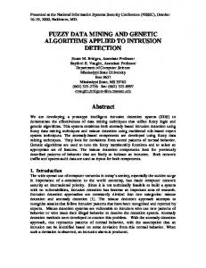
Fig. 1. Hydraulic flow model Baambrugge, The Netherlands (Witteveen+Bos consulting engineers).
conventional approach to this problem involves an arbitrary division of the data. Two other methodologies were successfully investigated by Bowden et al. (2002). In this publication the technique of Genetic Algorithms (GA) is used to reduce the artificially created datasets to smaller, optimised training datasets for the ANN.
(individuals) to the problem. The best solution is the maximum of a function. Through mutation and recombination (crossover) operations, possibly better solutions are generated out of the current set of potential solutions. This process continues until an acceptably good solution is found. In this paper the GA is used in combination with an ANN model. The ANN mimics a 1-D free surface flow drainage system in The Netherlands. An artificial dataset was constructed with discharge levels and discharge variations such that the discharges dataset overlap all flow conditions in the hydraulic computer model. The GA selects randomly five time periods from this initial dataset and puts them into a new dataset. The number of five time periods is a compromise between calculation time and calculation error. The ANN runs again with this new training set. This procedure is repeated until an optimal training dataset configuration is reached. The GA solves this problem in a reasonable time without restricting itself to local minima. In this paper the GA constructs an effective training dataset for an ANN networkbased model emulating a hydraulic flow model. From the available dataset usually a subset for training is carefully selected resulting in a suboptimal training datasets. The GA is used to change the training dataset where ranges of variables correspond with physical dimensions of 1-D natural limits of surface flow. The question is how to select the initial training set, how to construct a more optimal dataset and to improve the ANN’s training procedure in combination with the GA. The optimisation consists of a procedure which selects areas in the initial dataset that have a positive influence on the ANN’s performance. The hypothesis in this paper is that the initial training dataset contains sufficient input/output data for the ANN because it covers the total input space. However it is not known which part of the dataset contributes to adequate results, how many data is needed and in which sequence they should be placed. This is a complex optimisation problem. GAs have global optimisation capabilities and have advantages above other search techniques, including the ability to deal with qualitatively different types of domains, such as continuous variable domains and discrete variable domains. The GA will search in the artificial dataset for data that have positive influence on the training of the ANN.
2 Optimisation by Genetic Algorithms Genetic Algorithm is a search technique to find approximate solutions to optimisation problems. It is a global search technique and a particular class of evolutionary algorithms. From biological sciences, evolutionary processes have been translated to efficient search and design strategies. Genetic Algorithms use these strategies to find an optimum solution for any multi-dimensional problem (Goldberg, 1989). An optimal solution is however not guaranteed. Genetic Algorithms are search algorithms that mimic the behavior of natural selection. GAs attempt to find the best solution to a problem by generating a collection (population) of potential solutions Hydrol. Earth Syst. Sci., 10, 603–608, 2006
3
Flow model and methodology
In this paper the ANN simulates an existing hydraulic model of the drainage system of Baambrugge in The Netherlands which was created by Witteveen+Bos consulting engineers, Fig. 1. This model is built in Duflow which is software for modelling 1-D-channel flow. In Duflow the Saint-Venant equations are used for the free surface flow movements. Because of its open data structure Duflow is suitable for calculations in combination with other applications e.g. Matlab. The datasets consist of simulated discharges up and downstream www.hydrol-earth-syst-sci.net/10/603/2006/
R. G. Kamp and H. H. G. Savenije: Optimising training data for ANNs with Genetic Algorithms
605
Fig. 2. Input with stepped delay line to simulate history.
of a channel section and is simulated in a one-dimensional hydraulic network. ANN can simulate free surface flow (e.g. Bobovic and Abbott, 1997; Price et al., 1998; Bobovic and Keijzer, 2000; Minns, 2000; Dibike, 2002). This model has several discharge points and boundaries; there are also many rainfall-runoff areas connected. The input for the ANN is a discharge at the upper boundary. From that point the water disperses into the model. The output of the ANN is the discharge at a point, in the center of the model where boundary distortion is minimal. ANNs are capable to generalise system behavior from the training data (Anctil and Lauzon, 2004) and in a certain extent extrapolate (Shrestha et al., 2005). From this initial training data the GA selects five subsets with random start and endpoints. Consequently one observation can be used more than one time. The GA is free to choose the same start date for each subset. From some experiments the number of five subsets are chosen on considerations of calculation time and accuracy. Extra subsets did not give smaller errors and slowed down the calculation. Subsequently the ANN performs a run with this new training set. The error of the ANN is measured with the root mean squared-error (RMSE) of the simulated and target values. The target values are the simulated output of the numerical flow model. The ANN error was used as a fitness function value for the GA. The design parameters consist of start dates of the subsets. The parameter domain therefore equals the time period of the initial training dataset. No inequality constraints and equality constraints, nor a penalty function was used (Houck et al., 1995). The training set, consisting of new subsets, was used for the flow model to calculate new target values. The simulated and target values are compared and the GA generates, on the basis of the error, a new generation of training sets using selections, mutations, crossovers and other evolutionary methods. A cross validation set was used to prevent overfitting. The expectation is that the GA constructs a training set based on the original dataset and ensuring a minimum training error. www.hydrol-earth-syst-sci.net/10/603/2006/
Fig. 3. Example of starting index for five subsets in training data.
4
Model experiment
The input for the ANN is the upstream discharge model boundary which varies between 0.5 and 1.5 m3 /s to cover the input space. Within these limits the discharge model boundary frequency increases from days to hours in order to encapsulate enough floods of different durations. It is a sinfunction with a decreasing time period resulting in a quick oscillation at the end. The training target of the ANN is the discharge in the central area of the model. The target values are calculated in the numerical flow model. The input and output values will be used to design a data-driven model apart from the physically-based flow model. ANN are used because it is a widely used trend and proved to be an accurate regression method. Alternative methods are for example linear regression methods or model trees (Solomatine and Dulal, 2003). A stepped delay line is used to simulate stream flow dynamics. In a stepped delay line the input at time t until n steps in history Qt−n form the ANN’s input layer (see Fig. 2). The target values are the flow model’s output at time t. For the ANN we used two inputs; the 2nd and 7th time step of the upstream discharge model boundary in a stepped delay line. These steps were selected based on the cross-correlation graph of input and output data (see Fig. 7). The 2nd time step corresponds with the average travel time of a wave along the shortest route. In the cross-correlation graph there is platform at the 7th time step which could correspond to alternative ways for the wave to travel through the flow model. The ANN has two hidden layers with three neurons and five neurons respectively and an output layer with one neuron with Hydrol. Earth Syst. Sci., 10, 603–608, 2006
606
R. G. Kamp and H. H. G. Savenije: Optimising training data for ANNs with Genetic Algorithms Table 1. Testresults of optimised training set vs standard training (10 runs).
Fig. 4. Training set optimised by Genetic Algorithm.
Fig. 5. Distribution data points of optimised training sets in comparison to initial data set.
a linear transfer function. The neurons in the hidden layers have logsig transfer functions. The network structure, training algorithms, neuron functions and other ANN parameters are chosen on the basis of other hydraulic ANN model designs and experiences. It is a general problem that ANN has many design parameters that must be chosen and optimised. Therefore it is in general not straightforward to design a good structure for an ANN; a few rules of thumb for ANN in hydrinformatics were found by Zijderveld (2003). Other hydraulic ANN model designs and experiences were used as a first start. Another general problem of ANN is overfitting. Overfitting means that the training algorithm adjustst the weights of the ANN to fit every single data value in the dataset and at the same time decreases its capability to generelise future, new datasets. To prevent overfitting, a dataset from a situation for which the desired output Hydrol. Earth Syst. Sci., 10, 603–608, 2006
Testset
optimised training (rmse)
standard training (rmse)
Test 1 Test 2 Test 3
0.0085 0.0095 0.0043
0.0114 0.0134 0.0124
is known, is used in the training method. If the validation error increases while the training error steadily decreases then a situation of overfitting may have occurred and the training is stopped. It is necessary to test the ANN on test sets that relate to hydraulic situations. The method of randomization of test sets was not used because it would not allow blocks of data. For that reason the test set was created distinctly from the training set. The test sets represent different hydrological situations with variations in the hydrograph. The trained ANN will be used as an emulated flow model which, in concept, can simulate every flow condition. For this reason the testing was extended to three test sets, see Table 1. Each test set represents a situation with discharge variations with different time periods. These three test sets together cover most discharge variations of the flow model. In this paper the GA is used to optimise the training data to get a better trained ANN. The GA is trained for 30 generations each with 10 off-spring which is a small number. Some calculations with a higher number did not give lower errors. From the initial training set five subsets of equal length (150 data points) are selected. Only the starting point or starting index is chosen by the GA (see Fig. 3). The five subsets together form a new training set with new input/output time series and have a total length of 757 data points wich is half the length of the original training set. With the combined training set, the ANN makes a new calculation, resulting in a better performing ANN model (RMSE). Based on these results the GA starts the next run and chooses five new samples.
5
Conclusions
For many reasons sufficient and representative data is not always available. In this case we focused on a hydraulic flow model and presumed there is not enough data to train an ANN and decided to produce an artificial dataset. Therefore a dataset was composed regarding the properties of the flow network such as water depth, average discharge and timescales. With this dataset the ANN simulated the target model output which gave, as expected, poor results. The GA was used to improve the results of the ANN by optimising the original training set. The GA constructed a www.hydrol-earth-syst-sci.net/10/603/2006/
R. G. Kamp and H. H. G. Savenije: Optimising training data for ANNs with Genetic Algorithms
607
Fig. 7. Cross-correlation input and output discharge. Fig. 6. Frequency spectrum of optimised training set.
new training set by selecting different subsets from the original training set. The ANN was then trained again with this new training set. This was repeated until the GA found an optimal training set that performed much better than the initial training set. In this particular flow model it gave on average 39% better results when measured in RMSE. Figure 4 shows one of the resulting training sets. The sharp edges in the discharge indicate the borders of the subsets and have no special meaning. To take a closer look to the resulting dataset, Fig. 5 shows the distribution of the data points in comparison with the original, non optimised training set. A high density means the training set constructed with the GA chose that particular data point frequently. It shows which part of the original training set is represented by the optimised training set. The GA used data from the entire, original dataset consisting of 1489 data samples to find an optimised training set, except for the first 77 and the last 372 samples. In the last area the frequencies of the discharge is very high as shown in Fig. 3. The explanation for this is that in the flow model quick changes result in an almost constant discharge in the center of the model. The effect is that the relation between inputs and outputs is not ambiguous anymore. An ANN cannot handle this. As a result the GA did not select this area in the optimised training set. Slower changes were no problem for the ANN except for the very first samples where noise, induced by initial conditions, influenced the results. It is also interesting to look at the frequency distribution of the initial and the optimal frequency dataset as shown in Fig. 6. The initial dataset puts emphasis on waves with a time period of half a day. The optimised dataset has corrected this and put more emphasis on a broader spectrum with wave periods from 2.7 days to 14 h. Wave periods longer than 2.7 days (left part of the graph) were excluded in the optimised www.hydrol-earth-syst-sci.net/10/603/2006/
dataset. The GA created a more balanced training set. The optimized training and test sets correspond to a specific flow model and are not universal applicable for other flow models. For each new flow model a new initial training and test set is necessary. In this paper a GA was used to optimise the training data resulting in a better ANN simulating an existing hydraulic flow model in Baambrugge, The Netherlands. The resulting training data was built from five subsets selected by the GAs optimisation technique and resulted in an ANN which gives more accurate outputs. Further recommendation is to compare this method to other splitting algorithm methods. Edited by: D. Solomatine
References Anctil, F. and Lauzon, N.: Generalisation for neural networks through data sampling and training procedures with applications to streamflow predictions, Hydrol. Earth Syst. Sci., 8, 940–958, 2004, http://www.hydrol-earth-syst-sci.net/8/940/2004/. Babovic, V. and Keijzer, M.: Genetic programming as a model induction engine, J. Hydroinformatics, 2(1), 35–60, 2000. Babovic, V. and Abbott, M. B.: The evolution of equations from hydraulic data: Part I – Theory, J. Hydraulic Res., 35, 3, 1–14, 1997. Bowden, G. J., Holger, R. M., and Dandy, G. C.: Optimal division of data for neural network models in water resources applications, Water Resour. Res., 38(2), 1–11, 2002. Dibike, Y. B.: Model Induction from Data: Towards the next generation of computational engines in hydraulics and hydrology, IHE Delft, Delft, 2002. Doan, C. D., Liong, S. Y., and Karunasinghe, D. S. K.: Derivation of effective and efficient dataset with subtractive clustering method and genetic algorithm, J. Hydroinformatics, 7, 219–233, 2005.
Hydrol. Earth Syst. Sci., 10, 603–608, 2006
608
R. G. Kamp and H. H. G. Savenije: Optimising training data for ANNs with Genetic Algorithms
Feyen, L., V´azquez, R., Christiaens, K., Sels, O., and Feyen, J.: Application of a distributed physically-based hydrological model to a medium size catchment, Hydrol. Earth Syst. Sci., 4, 47–63, 2000, http://www.hydrol-earth-syst-sci.net/4/47/2000/. Goldberg, D. E.: Genetic Algorithms in Search, Optimization, and Machine Learning, Addison-Wesley Pub. Co., 1989. Hagan, T., Demuth, H. B., and Beale, M. H.: Neural Network Design, PWS Pub. Co., Boston, 1996. Haykin, S.: Neural Networks, a comprehensive foundation, Prentice Hall, New Jersey, 1999. Houck, C., Joines, J., and Kay, M.: A genetic algorithm for function optimization: a MATLAB implementation, NCSU-IE TR, 1995. Jolankai, G.: The Tisza River Project, Real-life scale integrated catchment models for supporting water- and environmental management decisions, Section 6 Report, Hungary, 2004. Minns, A. W. and Hall, M. J.: Artificial neural networks as rainfallrunoff models, Hydrol. Sci. J., 41(3), 399–417, 1996. Minns, A. W.: Subsymbolic methods for data mining in hydraulic engineering, J. Hydroinformatics, 2, 3–13, 2000. Price, R. K., Samedov, J. N., and Solomatine, D. P.: An artificial neural network model of a generalised channel network, Proc. 3rd Int. conf. Hydroinformatics, Copenhagen, 1998.
Hydrol. Earth Syst. Sci., 10, 603–608, 2006
Shannon, C., Moore, D., Keys, K., Fomenkov, M., Huffaker, B., and Claffy, K.: The internet measurement data catalog, Computer communication review, 35, 97–100, 2005. Shrestha, R. G., Theobald, S., and Nestmann, F.: Simulation of flood flow in a river system using artificial neural networks, Hydrol. Earth Syst. Sci., 9, 313–321, Solomatine, D. P. and Dulal, K. N.: Model trees as an alternative to neural networks in trainfall-runoff modelling, Hydrol. Sci. J., 48, 3, 399–411, 2003. de Vos, N. J. and Rientjes, T. H. M.: Constraints of artificial neural networks for rainfall-runoff modelling: trade-offs in hydrological state representation and model evaluation, Hydrol. Earth Syst. Sci., 9, 111–126, 2005, http://www.hydrol-earth-syst-sci.net/9/111/2005/. Whigham, P. A. and Crapper, P. F.: Modelling rainfall-runoff using genetic programming, Mathematical and Computer Modelling, 33(6–7), 707–721, 2001. Zijderveld, A.: Neural network design strategies and modelling in hydroinformatics, Ph.D. thesis, Delft University of Technology, Delft, 2003.
www.hydrol-earth-syst-sci.net/10/603/2006/