optimization of resource constrained project schedules by ... - CiteSeerX

ISSN 1392 – 124X INFORMATION TECHNOLOGY AND CONTROL, 2006, Vol. 35, No. 4

OPTIMIZATION OF RESOURCE CONSTRAINED PROJECT SCHEDULES BY GENETIC ALGORITHM BASED ON THE JOB PRIORITY LIST Leonidas Sakalauskas Vilnius Gediminas Technical University Sauletekio Str. 11, Vilnius

Gražvydas Felinskas Institute of Mathematics and Informatics, Faculty of Mathematics and Informatics Siauliai university, P.Visinskio Str. 19, Siauliai Abstract. Applications of information technologies are often related to making some schedules, timetables of tasks or jobs with constrained resources. In this paper, we consider algorithms of job scheduling related to resources, time, and other constraints. Schedule optimization procedures, based on schedule coding by the priority list of jobs, are created and investigated. The optimal priority list of jobs is found by applying the algorithms of local and global search, namely, Genetic Algorithm with constructed crossover, mutation, and selection operators, based on the job priority list. Computational results with testing data from the project scheduling problem library are given. Keywords: Resource constraint project, schedule optimization, Monte Carlo method, Genetic Algorithms, Variable Neighborhood.

1. Introduction

In this paper, we consider job scheduling and optimization algorithms related to resources, time and other constraints. In most cases, scheduling problems belongs to complexity class NP [19]. Optimal solution can be found using full binary recombination [9] or using methods based on ideas of branch and bound methods [2], etc. It is usually difficult or impossible to perform a full binary recombination in acceptable time, therefore, in order to schedule and optimize jobs, we may apply heuristic methods, based on priority rules [15], evolution process ideas [5,6], local search [12,17,22], variable neighborhood search [10,14], etc. We explore application of Genetic Algorithms [1,5,6,8,20] to schedule optimization because some investigations show that development of GA is a perspective trend to create efficient scheduling methods [6,12,14,17]. However, in the application of genetic algorithms important issues are to explore their efficiency depending on schedule coding and decoding, selection of parameter sets for a genetic algorithm. In this paper, we analyze the genetic algorithm based on the job priority list. Population forming, construction of operators for crossover, mutation and selection using the job priority list will be introduced and investigated. A more detailed discussion on the application of GA method to schedule optimization is presented in Sections 5.1 and 5.2.

Production scheduling is an important part of the production planning of many manufacturing companies. By scheduling it is possible to find the proper sequence to do the jobs and the proper schedule, when each operation of the job should be processed at each stage of the production process. A schedule is called feasible, if the precedence relations of the operations are maintained and the resource and other constraints are satisfied. Traditional scheduling methods, such as PERT (The Program Evaluation and Review Technique) and CPM (Critical Path Method), are not enough for production scheduling, because they consider infinite resources, i.e., they cannot take resource constraints into account [3]. Scheduling with infinite resources may give results, which are not feasible. In manufacturing industry, efficient methods to solve resource constrained scheduling problems are needed. Input data for such problems are a set of jobs, their durations, priority rules (successors, predecessors) and necessary resources. The aim is to find such schedule, which would meet the requirements of job priority relations, resource constraints, minimizing it by some criteria. In many cases this criterion is project’s finishing time.

412

Optimization of Resource Constrained Project Schedules by Genetic Algorithm Based on the Job Priority List

Computational results are given using data sets from the project scheduling problems library (PSPLib) [18,21]. A more detailed discussion about PSPLib, testing data sets and solutions is given in Section 4.

The objective function defines the finishing time of the whole job project, inequality (1) describes priority relations, and the inequality (2) requires to pay heed to resource constraints.

2. Schedule optimization problem

3. Schedule coding and decoding

Resource constrained project scheduling problems (RCPSPs) [13] involve assigning jobs or tasks to a resource or a set of resources with limited capacity in order to meet some predefined objective. Input data for schedule planning and optimization are set of jobs and their durations, description of resource constraints and a set of priority relations. Let‘s denote by J = {0,1,...,n ,n + 1} a set of jobs,

Efficiency of schedule optimization algorithm depends on solution coding [4,10,14]. In this paper, we analyze job scheduling problems under resource constraints with solution coding in a shape of a priority list [15,16]. The job priority list b = (0,b1 ,b2 ,...,bn ,bn +1 ) can be determined by jobs’ starting times vector s, where sbi ≤ sb j if i < j . It is very important that this vector of starting moments must meet priority relations and resource constraints. On the other hand, for a given priority list, we can find the vector of job starting times concerted with the priority list and initial priority constraints. For this we use serial decoder described in Section 3.2. At first, we must be sure that the priority list is concerted with priority constraints. Let’s call the priority list from which we can find a vector of jobs’ starting times concerted with priority relations as a permissible priority list. Using a set of priority relations, we can check whether the solution is permissible or not. For any permissible job priority list, by applying the serial decoding procedure, we can determine jobs’ starting times vector which may minimize a project finishing time, according to priority relations, resource constraints, and a given job priority list. The constructed algorithm should enable us operating with job priority lists to search such job priority list which would correspond to solution (maybe optimal) of the problem (1),(2).

where jobs No.0 and No.(n + 1) are dummy and mean the beginning and the end of the whole project, d j , j ∈ J – duration of the j th job, d j ≥ 0 , j ∈ J – non-negative numbers and d 0 = d n+1 = 0 . We can define priority relations in a set J as a set of pairs C = { (i, j) | i must be executed before j } . Let‘s denote a set of resources by K = {1,..., m } . All resources are renewable and non-additive – at every moment we can use fixed amount of each type of resources, remains are gone. Let’s assume amounts of resources R k > 0, k ∈ K , be constant. Let‘s denote the starting moment of the j th job by s j ≥ 0 , and correspondingly r jk ≥ 0 - amount of the k th resource, needed for performing this job. Let’s assume that the started jobs must be performed without breaks. Then the finishing time of the j th job can be defined as

c j = s j + d j . The problem of schedule making may be reduced to the problem of finding a vector s = (s 0 , ... , s n +1 ) of jobs’ starting time which would meet priority and resource requirements and would minimize a certain objective function. An objective function may reflect the economical outlay (outgoing), yield (incoming), finishing time, and etc. Project finishing time is one of the most analyzed schedule optimality criteria which will be applied in this paper. Let‘s denote by A(t) = { j ∈ J | s j ≤ t < c j } a set

3.1. Determination of admissibility of the job priority list Let‘s analyze admissibility determination of the job priority list. Let’s introduce the binary relation vij = 1, if (i, j ) ∈ C, vij = 0 , matrix V = (vij ,1 ≤ i , j ≤ n ) ,

if (i , j ) ∉ C , related with a set of priority constraints and define a full priority relations’ matrix G = g ij ,1 ≤ i , j ≤ n . This matrix describes all chains

(

of jobs which were started but not yet completed at the time moment t. Let T ( s ) stand for the project finishing time, T( s ) = c n +1 . After these definitions we can formulate the problem of minimization of the objective function T ( s ) .

of priority relations. So, g kj = 1 if it is possible to find such a sequence of index pairs that ( k , k1 ) ∈ C , ( k1 , k 2 ) ∈ C , ..., ( kl , j ) ∈ C . The matrix V has the following property: vij = 1 ⇒ v ji = 0 . The matrix G

Find min T( s ) , subject to:

has this feature as well. The priority list is permissible if bi ,b j are the components of b, and

s

ci ≤ s j , ( i , j ) ∈ C ,

(1)

i < j ⇒ g b j ,bi = 0 applies for any pair ( bi ,b j ) . For

sj ≥ 0, cj =sj +d j , j∈J ,

∑ rkj ≤ Rk , k ∈ K , 0 ≤ t ≤ cn +1

)

determination of full priority relations’ matrix,

(2)

j∈ A(t )

413

L. Sakalauskas, G. Felinskas

according to the given set of priorities C , we can use the following algorithm:

4. Project scheduling problem library PSPLib 4.1. Description of the PSPLIB library

FOR i=1 TO n DO FOR j=1 TO n DO g(i,j)=v(i,j); FOR i=1 TO n DO FOR j=1 TO n DO IF v(i,j)=1 THEN FOR k=1 TO n DO IF g(j,k)=1 THEN g(i,k)=1;

This library [18,21] contains different problem sets for various types of resource constrained project scheduling problems as well as optimal and heuristic solutions. The data sets may be used for the evaluation of solution procedures for single- and multi-mode resource-constrained project scheduling problems. The instances have been generated by the standard project generator ProGen. Researchers may download the benchmark sets to evaluate their algorithms, and they may send their results to be added to the library. The main parameters are given in the following sections.

3.2. The serial priority list decoder

Let‘s analyze the serial decoding procedure constructed for the priority list decoding. This procedure computes the early starting moments of jobs, according to jobs’ priority list concerted with priority relations, and resource constraints. In schedules obtained in such way, none of jobs can be started earlier than calculated time, without violation of priority relations or resource constraints. We can call such schedules active ones [14]. The optimal schedule is considered to be active as well. Let‘s describe the algorithm for determination of the active schedule. Step 1. Set initial s 0 = c0 = 0 . Let i = 1 .

4.2. Kinds of solutions and instance sets

For each instance set xyz of the mode mm, one can find an archive file called xyz.mm.tgz that includes the complete set of instances. E.g., the 480 single mode problems with 30 jobs are in the file j30.sm.tgz. Files containing heuristic solutions, optimal solutions and lower bounds can be found in the archive. They are grouped like the benchmark instances by their mode (single, multi or other) and by the number of jobs (30, 60 etc.). Detailed description of solutions format can be found in [21].

Step 2. Assume that starting times of the first jobs from the priority list have already been

( i −1)

determined. So, we know all sb j ,cb j , j ≤ i − 1 .

4.3. Parameter Settings

Let’s denote the moment Ti = max( max cbl , max sbl ) g bl ,bi =1 0 ≤ l ≤ i −1

There are a lot of RCPSP instances (input data sets, best known solutions) in the PSPLIB. More precisely, 480 samples for every problem with n=30, 60 and 90 jobs, and 600 samples for n=120. The number of resource types is 4. All samples are divided into classes. There are 10 samples in every class, generated using random numbers generator with fixed values of three parameters: • NC ∈ { 1.5;1.8; 2.1 } – averaged number of jobspredecessors for every job. • RF ∈ { 1;2;3;4 } – number of resource types, needed for every job. • RS ∈ { 0.2; 0.5; 0.7;1.0 } – amount of given resource at every moment; Value RS = 0.2 matches examples with minimum amount of given resources, enough for solving problem; Value RS = 1 matches the case without resource constraints. It is known that values of parameters RF = 4 , RS = 0.2 match hard enough classes. Their identifications are j3013, j3029, j3045 with value n = 30 ; j6013, j6029, j6045 with value n = 60 ; j12016, j12036, j12056 with value n = 120 . Each triplet of these identifications matches values NC = 1.5;1.8; 2.1 accordingly.

0 ≤ l ≤ i −1

The starting time of the next job is equal to latter moment, provided the resource constraints are met:

sbi = Ti if

∑

j∈ A( Ti )

rk j ≤ Rk ,1 ≤ k ≤ K .

If resource constraints are not met, then the starting time of this job is equal to finishing time of the first completed job, when resource constraints are met: sbi = min cb j ∑

l∈ A( cb j )

rkl ≤ Rk ,1≤ k ≤ K , cb j >Ti ,1≤ j ≤i −1

The finishing time of bi -th job can be calculated simply:

cbi = sbi + dbi Step 3. If i = n , then { T ( S ) = cbn + d n +1 , end of

the algorithm}, else { j = j + 1 , go to step 2}. It is easy to notice that it is necessary to make O( n ⋅ m ) elementary operations for performing step 2 of the algorithm [14]. Therefore, the computational complexity of the decoding procedure is O( n 2 ⋅ m ) .

414

Optimization of Resource Constrained Project Schedules by Genetic Algorithm Based on the Job Priority List

Here we give a description of parameters settings for mostly used single-mode RCPSP. (Detailed description of all parameters is given in [18]).

4.4. Characterization of the Benchmark Instances

Currently, two benchmark sets are available for the SMRCPSP and 25 benchmark sets for the MMRCPSP. Input parameters are grouped into three classes: first, fixed parameters which are constant for all benchmark sets, second, base parameters mainly one of which is adjusted individually for each benchmark set, and third, variable parameters which are systematically varied within each benchmark set.

Table 1. Fixed Parameter Setting - SMRCPSP and MMRCPSP

P1R

P2R

P1N

P2N

ε NET

ε RF

0.00

1.00

0.00

1.00

0.05

0.05

Table 2. Base Parameter Setting (SMRCPSP)

min max

J

Mj

dj

R

UR

QR

N

UN

QN

S1

Sj

PJ

Pj

30 30

1 1

1 10

4 4

1 10

1 2

0 0

0 0

0 0

3 3

1 3

3 3

1 3

Table 3. Variable Parameter Settings (SMRCPSP) Parameter

NC

1.50

Levels 1.80 2.10

RFR

0.25

0.50

0.75

1.00

RS R

0.20

0.50

0.70

1.00

The instances for the SMRCPSP have been generated with the fixed, base, and variable parameter settings given in Tables 1 to 3. Utilizing a full factorial design of the variable parameters NC , RFR and RS R with 10 replications per triplet < NC , RFR , RS R > we can generate a total of 3 × 4 × 4 × 10 = 480 benchmark problems for each set.

Table 4. Instance Sets - SMRCPSP Instance set P

J30 J60

[1..48] [1..48]

E

[1..10] [1..10]

Type SM SM

Varied base parameter table 2.

Variable setting

Number of instances

Solution obtained by

J min = J max = 30

Table 3

480

opt.

J min = J max = 60

Table 3

480

hrs.

5. Schedule optimization algorithms

Table 4 provides a summary of the instances produced. The first column (instance set) gives the prefix of the file names the instances are stored under; the second column (P) displays the range of the cell index, reflecting the combination of the variable parameters. The third column (E) specifies the range of the instance index within a cell. The 4th column abbreviates the acronym SMRCPSP to SM and serves as the suffix of the filenames. The 5th column shows the varied base parameters, here the number of activities which has been set to 30 and 60, respectively. The 6th column references to the table with the variable parameter levels employed. The 7th column displays the number of instances within the benchmark set. Finally, the 8th column shows how solutions of the benchmark sets have been obtained. A complete file name, e.g., J301210.SM, corresponds to instance set J30, variable parameter combination 12, and problem number 10 of the SMRCPSP. The level of the variable parameter settings for each parameter cell index can be found in the files J30PAR.SM and J60PAR.SM, respectively. Optimal objective function values for the instances of the J30 benchmark set have been obtained by and are documented in the file J30OPT.SM. Currently, the instance set J60 cannot be solved by exact solution procedures. For this, heuristic methods must be used.

5.1. Description of the Genetic Algorithms

For schedule optimization, we can apply evolutionary algorithms such as Genetic Algorithm [5,6]. GAs owe their name to an early emphasis on representing and manipulating individuals at the level of genotype. In Holland’s original work [11], GAs were proposed to understand adaptation phenomena in both natural and artificial systems and they have three key features that distinguish themselves from other computational methods modeled on natural evolution: 1. The use of bit string for representation; 2. The use of crossover as the primary method for producing variants; 3. The use of proportional selection. Genetic Algorithms are the most popular technique in evolutionary computation research. In the traditional genetic algorithm, the representation used is a fixed-length bit string. Each position in the string is assumed to represent a particular feature of an individual, and the value stored in that position represents how that feature is expressed in the solution. Usually, the string is “evaluated as a collection of structural features of a solution that have little or no interactions” [1]. The analogy may be drawn directly to

415

L. Sakalauskas, G. Felinskas

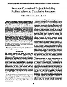
genes in biological organisms. Each gene represents an entity that is structurally independent of other genes. The more classical reproduction operator used is one point crossover, in which two strings are used as parents and new individuals are formed by swapping a sub-sequence between the two strings (see Figure 1).

Step 1. Generate M permissible priority lists ( M = 40 , 20 , ... ). Construct the matrix BP = bij ,

( )

1 ≤ i ≤ M , 1 ≤ j ≤ N , N – number of jobs, M – number of lists in the population. IT = 1 . T best = T ( any priority list ) .

( T best best achieved value of the objective function through evolution). Step 2. (Crossover) In each IT th iteration perform the crossover procedure with every pair of priority lists.

Crossover point

Let b' and b* be priority lists (“parents“). Select position w randomly. From two permissible priority lists b' = ' (b1 , ..., bw' , bw' +1 , ..., bN' ) and b* = ( b1* ,...,b*w ,b*w+1 ,...,b*N )

Figure 1. Bit-String Crossover of Parents a) and b) to form Offspring c) and d)

Another popular operator is bit-flipping mutation, in which a single bit in the string is flipped to form a new offspring string (see Figure 2).

we get two new priority lists b'' and b** (“children”). Let’s construct b'' = ( b1' , ...,b'w ,b*k1 , ...,b*k ,N − w ) , here b*k1 , ...,bk* ,N − w – the components of vector b* that

were left after elimination of of vector b' ( b1' , ...,b'w ) from order of the components in Analogously construct

Figure 2. Bit-Flipping Mutation of Parent a) to form Offspring b)

A great variety of other crossover and mutation operators have also been developed. A primary distinction that may be made between the various operators is whether or not they introduce any new information into the population. Crossover, for example, does not while mutation does. All operators are also constrained to manipulate the string in a manner consistent with the structural interpretation of genes. For example, two genes at the same location on two strings may be swapped between parents, but not combined based on their values. Traditionally, individuals are selected to be parents probabilistically based upon their fitness values, and the offspring that are created replace the parents. For example, if N parents are selected, then N offspring are generated which replace the parents in the next generation. These methods are used to solve various design optimization problems (including discrete design parameters, real parameters). Early applications of GAs are optimization of gas pipeline control, structural design optimization [8], aircraft landing strut weight optimization [20], keyboard configuration design [7], etc.

the first w components vector b* . Preserve the the resulting sequence. b** = (b1* , ..., bw* , bk' 1 , ...,

bk' , N −w ) .

Note that new priority lists b' and b* are permissible too, because all precedence relations are kept. Perform this crossover procedure with all pairs of rows of matrix BP (M/2 pairs). BP crossover  → BC . Step 3. (Mutation) In each IT th iteration perform the mutation procedure (theoretically, we give a chance to construct any priority list from all solution space). With the given probability pp, select chromosomes (priority lists) for mutation procedure. After this selection, perform mutation procedure with these priority lists (rows of matrix BC ) in the following way: Generate random numbers l and q , l ≠ q , 1 ≤ l , q ≤ N . With the probability p = 0,5 perform one of

the following operations: move the q th job before the l th job (shift) or swap the q th and l th jobs. If new priority list after these operations is not permissible,  → BC MUT . cancel the operation. BC mutation Step 4. (Selection) From M + M priority lists (“parents“ and “children“) we must select only M priority lists. (We can select and leave only priority lists with smallest values of the objective function Z = T ( b ) . Different methods of selection are described in [6]) After merging matrices BP and BC , we get new a matrix BPC , with dimensions 2M × N .

5.2. Schedule optimization using the Genetic Algorithm

We applied the genetic algorithm with the constructed crossover, mutation, and selection operators, based on permissible job priority lists. In such a way we bypassed the procedures of coding and decoding from the binary code, which can generate impermissible priority lists. [1,6,8] Let us write such GA algorithm:

416

Optimization of Resource Constrained Project Schedules by Genetic Algorithm Based on the Job Priority List

simulation. The constructed algorithm was tested on data sets from the project scheduling problems library PSPLib.

Select lists b' and b* at random from the matrix *

BPC . Calculate Z1 = T (b ) and Z 2 = T ( b ) . If '

Z1 < Z 2 , then leave priority list b' and remove b* . Otherwise, leave b* and remove b' . After M such “duels” we again get a matrix with dimensions M ×N .

6.1. Optimization by Genetic Algorithm and efficiency dependence on parameter settings

To investigate the convergence rate of the objective function value to global minimum or to the best known value, using the Genetic Algorithm, we took several data sets of different dimension (the number of jobs) and complexity (different amount of necessary resources and different number of precedence relations). Averages of the convergence rate were calculated from 100 modeling experiments for data sets with 30 and 60 jobs and from 10 modeling experiments for data sets with 90 and 120 jobs. In Tables 5, 6, 7, Avg. denotes Average, it. – iterations.

Step 5. Find the best solution T* = min T(b i ) in 1≤i ≤ M

the chromosomes population. If T * < T best , then update not only value, but the best solution as well T best = T * . Step 6. If IT = ITmax , then stop, otherwise set IT = IT + 1 and go to Step 2.

6. Modeling results We investigate the efficiency and convergence rate of constructed genetic algorithm by statistical

Table 5. Convergence rate of the objective function value to global minimum using Genetic Algorithm (3 different instances of input data sets from PSPLib, 4 different parameter settings for GA, number of jobs j=30) data set #1

data set #2

data set #3

30 41

30 38

30 63

Number of jobs Known optimum of Objective Function Avg. number of it. for optimal solution

83

15

21

18

162

42

35

18

24

6

8

5

Mutation probability Pmut

0.1

0.1

0.3

0.3

0.1

0.1

0.3

0.3

0.1

0.1

0.3

0.3

Number of individuals in population

20

40

20

40

20

40

20

40

20

40

20

40

3.17

1.38

0.99

1.33

6.04

3.28

1.48

1.58

1.51

0.65

0.48

0.61

Avg. time for finding optimum, s.

Table 6. Convergence rate of the objective function value to the best known value using Genetic Algorithm (3 different instances of input data sets from PSPLib, 4 different parameter settings for GA, number of jobs j=60) data set #1

data set #2

data set #3

60 77

60 59 892

60 76 141 38

57

0.1

0.1

0.3

Number of jobs Best known value of Objective Function Avg. number of it. for solution

110

92

45

32

358

188

345

175

Mutation probability Pmut

0.1

0.1

0.3

0.3

0.1

0.1

0.3

0.3

Number of individuals in population Avg. time for finding best known value, s.

0.3

20

40

20

40

20

40

20

40

20

40

20

40

23.8

39.9

10.7

14.4

77.8

80.7

75.3

76.1

193.4

60.6

8.3

24.8

Table 7. Convergence rate of the objective function value to the best known value using Genetic Algorithm (1 instance of input data for j=90, 2 instances for j=120, 4 different parameter settings for GA) data set #1

data set #1

Number of jobs Best known value of Objective Function Avg. number of it. for solution Mutation probability Pmut

* 0.1

* 0.1

944 0.3

452 0.3

Number of individuals in population

20

40

20

Avg. time for finding best known value, s.

*

*

636

90 67

data set #2

* 0.1

120 99 * 894 0.1 0.3

* 0.1

120 111 * * 0.1 0.3

442 0.3

436 0.3

40

20

40

20

40

20

40

20

40

623

*

*

1388

1368

*

*

*

1350

* - best known value of the objective function not reached (during modeling, max 1000 iterations were done).

better results we can reach using Pmut =0.3 and the smaller number of chromosomes in population (20).

Computational results show us that in cases with lower problem dimension (number of jobs 30 or 60)

417

L. Sakalauskas, G. Felinskas

Too low mutation probability does not guarantee enough recombination of priority lists and the big number of chromosomes in the population can take more computational time (Table 5 and Table 6). In cases with higher problem dimension (number of jobs 90 or 120) with too low mutation probability and number of chromosomes in population, finding the optimum can take too much computational time (Table 7). Although with the higher number of chromosomes (40) it takes more computational time for each iteration, better recombination of solutions finally gives us better results of overall computational time, needed for finding best known objective function values.

[4] G. Felinskas, L. Sakalauskas. Pareto type models in simulated annealing algorithms. Lithuanian Mathematical Journal, ISSN 0132-2818, 2003, T.43, special volume, 573-578 (in Lithuanian). [5] Genetic algorithms. http://www.pcai.com/web/ai_info/genetic_algorithms. html, 2000. [6] N.N. Glibovec, S.A. Medvidj. Genetic algorithms and their application to project scheduling problem solving. Cybernetics and system analysis, 2003, No.1, 95-108 (in Russian). [7] D.E. Glover. Experimentation with an adaptive search strategy for solving a key-board design/configuration problem. Doctoral Dissertation, University of Iowa, 1986. [8] D.E. Goldberg. Genetic Algorithm in Search, Optimization and Machine Learning. Addison-Wesley Publishing Company, Inc., Reading, Massachusetts, 1989. [9] Gray code from Wikipedia, the free encyclopedia. http://en.wikipedia.org/wiki/Gray_code. [10] P. Hansen, N. Mladenovic. An introduction to variable neighborhood search. Metaheuristics: Advances and Trends in Local Search Paradigms for Optimization, Kluwer, 1999, 433-458. [11] J.H. Holland. Adaptation in Natural and Artificial Systems. University of Michigan Press, Ann Arbor, 1975. [12] H.H. Hoos, Th. Stutzle. Stochastic Local Search. Foundations and Applications, Morgan Kaufmann, Elsevier, 2004. [13] R. Klein. Scheduling of Resource-Constrained Projects. Kluwer Academic Publishers, 2000, 369. [14] J.A. Kocetov, A.A. Stoliar. Application of alternating environments to approximate solving of RCPSP. Discrete analysis and operation research 2003, Ser.2, Vol.10, No.2, 29-55 (in Russian). [15] R. Kolisch. Efficient priority rules for the resourceconstrained project scheduling problem. Journal of Operations Management, 1996, No.14, 179-192. [16] R. Kolisch. Serial and parallel resource-constrained project scheduling methods revisited: Theory and computation. European Journal of Operational Research, 1996, Vol.90, No.2, 320-333. [17] R. Kolisch, S. Hartmann. Project scheduling: Recent models, algorithms and applications. Kluwer, Amsterdam, 1999, 147-178. [18] R. Kolisch, A. Sprecher. PSPLIB – A project scheduling library. European Journal of Operational Research, 1996, Vol.96, 205-216. [19] R. Lassaigne, M. de Rougemont. Logic and Complexity. Zara, Vilnius, 1999, (in Lithuanian). [20] A.K. Minga. Genetic algorithms in aerospace design. The AIAA Southeastern Regional Student Conference, Huntsville, AL, 1986. [21] PSPLIB - A project scheduling library. http://www.bwl.uni-kiel.de/Prod/psplib/, 1996. [22] S. Voss. Meta-heuristics: The State of the Art. Local Search for Planning and Scheduling, LNAI 2148, 2001, 1-23.

7. Conclusions and further research 1. Algorithms for planning and optimizing schedules of jobs with resource constraints, based on schedule coding by the job priority list and the serial priority list decoding procedure, were discussed in this paper. This kind of schedule coding generally allows us to apply several heuristic optimization methods. 2. Genetic algorithm based on the priority list for RCPSP optimization has been created. This algorithm has been investigated and compared by statistical modeling, while using data sets and known solutions from the PSP Library. 3. The testing results show that the created algorithm is able to find the best known solutions of problem instances from the PSP Library while using computational time acceptable in practice. 4. The computational results with the examples from the PSP Library have shown that GA performs better with certain mutation probability (Pmut = 0.3). With an increase in the number of jobs in the schedule, population of chromosomes must be increased as well. 5. Future research plans include comparison of genetic algorithms for RCPSP, based on the priority list with other heuristic approaches, namely, Simulated Annealing, Tabu Search, Scatter Search, etc.

References [1] P.J. Angeline. Genetic programming’s continued evolution. Chapter 1 in K.E. Kinnear, Jr. and P.J. Angeline (Eds.), Advances in Genetic Programming 2. Cambridge, MA: MIT Press, 1996, 1 -20. [2] P. Brucker, S. Knust, A. Schoo, O. Thiele. A branch and bound algorithm for the resource-constrained project scheduling problem. European Journal of Operational Research, 1998, Vol.107, No.2, 272-288. [3] B.P. Douglass. Software Estimation and Scheduling. http://www.techonline.com/community/ed_resource/te ch_paper/5947.

Received August 2006.

418