site selection: one pertains to the estimation of variogram and the second concerns ... extends that of Russo 1-1984], who discussed the optimization of location ...
WATER
RESOURCES
RESEARCH,
VOL.
23, NO.
3, PAGES
496-500,
MARCH
1987
Optimization of Sampling Locations for Variogram Calculations A. W. WARRICK
Department of Soil and Water Science,The University of Arizona, Tucson D.
E. MYERS
Department of Mathematics, The University of Arizona, Tucson
A method is presentedand demonstratedfor optimizing the selectionof sample locations for variogram estimation. It is assumedthat the distribution of distance classesis decided a priori and the problem thereforeis to closelyapproximate the preselecteddistribution, although the dispersionwithin individual classescan also be considered.All of the locations may be selectedor points added to an existing set of sites or to those chosen on regular patterns. In the examples, the sum of squares characterizing the deviation from the desired distribution of couplesis reduced by as much as 2 orders of magnitude between random and optimized points. The calculations may be carried out on a microcomputer. Criteria for what constitutesbest estimators for variogram are discussed,but a study of variogram estimatorsis not the object of this paper.
INTRODUCTION
Geostatistics is applicable to a variety of problems in hydrology and soil science. The variogram is the key function which quantifies the interdependence of sampling locations; i.e., two samples from nearby locations tend to be more alike than two taken from widely separate locations. One of the first stepsin the application of geostatisticsis the determination of the variogram. The variogram must, in general, be estimated from the data, and then a model is selected
class is given. The schememay be used either for choosing a complete set of points or to select additional points in order to augment an existing set of points or those of a specifiedpattern, such as along a transect or on a regular grid. The complete problem of what constitutesthe best selectionof points is not our objective; however, we will suggestappropriate criteria
for that
characterization.
It
is assumed
that
the ideal
distribution is decided a priori. We are simply developing a schemeto meet prespecifiedconstraints.
which satisfiesthe positive definite condition, as well as being REVIEW OF THEORY compatible with the data in some appropriate sense,such as Let Z(x) denote the value of the characteristic or attribute cross-validation.Whether the sample variogram is used or one of interest at the point x' x could be a point on a transect or of other proposed estimators, it is necessaryto generate paired differences. The characteristicsof the set of paired differences in an area or in a volume. If Z(x) is modeled by a random function satisfyingthe intrinsic hypothesisthen the variogram are crucial to the efficiency of the variogram estimator. In turn, these characteristicsare strongly influenced by the sam- is given by pling plan. 7(h) = (1/2) Var [Z(x + h) - Z(x)] For any sampling exercise, the location of sites is a con= (1/2)E{[Z(x + h) -- Z(x)] 2} (1) sideration. There are two obvious considerationsfor sample site selection:one pertains to the estimation of variogram and If x• .... , x• are N sample locations then the sample variothe second concernsthe use of data for kriging but assumes gram is given by the variogram has previously been determined. In the latter n(h) case, the kriging variance can be used to construct an objec7*(h) = [1/2n(h)] • [Z(xi + k) - Z(xi)]2 (2) tive function and that problem has attracted the interest of a i=1 number of authors [cf. Burgesset al., 1981; McBratney and where Webster, 1983]. We shall only consider the problem of variogram estimation and only the problem of site selection,rather Ihl- e • Ikl • Ihl + e (3) than that of the derivation
of alternative
estimators.
Our work
extends that of Russo 1-1984],who discussedthe optimization of location selectionbased on homogeneity within classesof a given lag tolerance. Bresler and Green [1982] discussthe use of randomly generated sample locations to ensure that the distribution of classnumbers be as close to uniform as possible.
The objective of this paper is to develop a method to choose sample locations, optimized with respectto prespecifieddistributions of couples for the distance classes.A second criterion based on the dispersion of separation distances within each Copyright 1987 by the American Geophysical Union. Paper number 6W4737. 0043-1397/87/006W-4737505.00
On --• < OR < On + •
(4)
with Ihl being the length of the vector h; 0n the direction of h; 2e the width of the distance class; and 26 the width of the
angle window. Finally, n(h) is the number of pairs (xi q- k, xi) satisfyingthe distanceand angle conditions. The y*(h) is an unbiasedestimator of y(h) for each h, but, as is noted by Cressie and Hawkins [1980] and Armstrong and Delftnet [1980], it is not robust. Since it is not our intention to derive
a new estimator
but
rather
to enhance
known
esti-
mators by appropriate sampling patterns, we will focus on the sample variogram. The results are equally relevant for others that have been proposed. Davis and Borgman [1978, 1982] obtained a central limit
property for y*(h) assumingfourth-order propertieswhich sug496
WARRICK AND MYERS: VARIOGRAM CALCULATIONS
No I t. er'at. i one H-O N-30 +
400.
H-O
4. The average of the angles in each class should be close to the plotted angle. 5. The variance of the anglesin each classshould be small. It should be noted that a regular grid will tend to ensure conditions 2-5, but N will have to be large to satisfy condition 1. An alternative choice, random selection of the sample locations does not ensure any of the five conditions.
N-30
• 2oo. B
5OO
400.
! t. er'ot.l N-30
14-O
one
+
Supposef•*, "', fNc* is a prespecifieddistribution and we wish to obtainf•, .-., f•c closeto this distribution while satisfying 2-5 to some degree. For example, we might take all f•* = N(N- 1)/(2NC). With this in mind, we define SS to be
. +..•:
%+
E
:+'
+
-,' 200. >-
-•
++
+
500
0
C O.
.
,
,
O.
i
,
200. X
,
.
400.
"•
+ + -*'+:1: '• +%,•*.
+ + .,.•;• ,
i
O.
I terot,
#-0 ,
,
200.
minimized:
J one NC
N-30 i
,
497
'•'
NC
NC
SS= a •. w,(f•* _f•)2 + b • rn,i+ c •'. rn2,
,
400.
i=1
i=1
(6)
i---1
X
(m)
Fig. l. Distribution of points initially (a), after 100 iterations (b), and after 500 iterations (c) for example 1. Also presented are results for example 3 based on minimum moments about classmean results (d) after starting with Figure lb.
where w•, ..., WNC;a, b, and c are user-selectedweighting coefficients;the rn• are absoluteor secondmoments of the distanceclasses;and the m2i are the absolute or secondmoments for the angle classes.For the most part, the isotropic case is considered, and c is taken as 0. In addition, we will
gests that n(h) should be as large as possible. The problem is complicated by the fact that ?(h) must be estimated for many values of h and not just one; i.e., it is the function that must be estimated and not just the values of ?(h) at a finite number of points. Without additional multivariate distributional assumptions for Z(x), statistical inference is not possible. It is known that the behavior of ?(h) is most critical for Ihl small; hence n(h) should be large for Ihl small. In addition to a large number of h's, in general, a number of angle classesmust be
concentrate
considered.
mation might be used in choosing the h/s and the desired
After
these choices
of h and of directional
classes
are made, the site locations must be chosen. One would like to make the selection to optimize one or more desirable characteristics, such as the confidence level and confidence width for
estimatesof ?(h). In general, this is not possible without additional distributional assumptions and it does not guarantee optimal estimation of the variogram function. We will consider then conditions which are clearly necessaryor desirable or Supposethen that N locations are to be selected,then there are N(N - 1)/2 pairs. In general,the number of pairs for short lag distancesis small as is the number for large lag distances. The greatest number of couples occurs at approximately half the maximum separation distance. Moreover, there may be excessivedispersion within each distance-angle class,resulting in excessiveaveraging. Without loss of generality assumedistance classesare defined by 0, h•, ---, hNo whre NC is the number of classes.For the isotropic case the hi's are simply distances.For the classhi, let f• denote the number of pairs; i.e.,f• = n(hi).It is immediatethat
The casewi = l/a, all f•*'s are the same,and b = c - 0 is the same as the criterion given by Bresler and Green [1982]. The case where a - 0, b - 1, and c - 0 is very nearly the criterion used by Russo [1984]. We can equally well assumethat M sites have already been selected; 0 < M < N and hence consider this option. Note that no a priori assumptions are made about the variogram type nor about the range of dependence although this infor-
distribution for the number of pairs. While we have focused on the use of the sample variogram, conditions 2-5 are still relevant for all of the other variogram estimators that have been proposed. EXAMPLES AND CALCULATIONS
For our first two examples we will choose a = 4[N(N
hence we can only apportion the pairs between classesin some optimal way. We can now identify a number of properties that are necessary or desirable but which, in general, are in conflict, as follows.
1. For each distance-angle class, the number of pairs should be as large as possible,particularly for short distances. 2. The average of the distances in each class should be close to the plotted lag. The
variance
of the distances
minimum
in each
class should
be
value of SS is as follows.
1. Specify M fixed points at x•, x 2, --., x M and the total number of points N. 2. Specify the number of classesof couples NC along with
TABLE 1. Distribution of Couple Separation Distancesfor Examples 1-3 Iterations
Example 1
Example 2
Example 3
Class, m
NC
small.
0.
-- 1)]-2, wi = 1, and b = c = 0 in (2). A procedureto find a
both.
3.
on the case b -
0
100
500
0
100
500
0
100
500
0-20
8
31
40
2
11
17
31
25
25
20-40
12
47
45
6
15
18
47
25
29
40-60
20
32
41
10
13
17
32
30
30
60-80
18
32
42
21
12
19
32
33
46
80-100 100-120
27 20
36 41
42 44
17 45
33 61
36 41
32 23 44 30 201 0.026
31 39 41 50 55 0.0038
44 41 41 42 13 0.0002
21 42
228 0.037
43 45 23 22 157 0.027
31 39 41 50 55 1.0
28 30 27 36 35 42 124 0.886
51 25
120-140 140-160 160-180 180-200 >200 SS
32 51 31 46 23 26 155 0.020
mavg
5.1
4.9
5.2
5.5
5.5
5.4
4.9 4.3
19 24
N = 30.In eachcase,f•* = 43.5for everyclass.
28 28 25 25 123 0.80
3.9
498
WARRICK AND MYERS: MARIOGRAMCALCULATIONS
the classlimits hx, h2, .-- , hNcand the desirednumberf• for each class or the fraction of the total in each class(f•/[N(N - •)/2]).
ations the result is as in Figure lb with $$ = 0.0038. The points are selectedcloser together and give a very even distribution
of class sizes. After
500 iterations
the distribution
of
3. Choose N--M random points giving x•t+x, '", xN points appear visually about the same (Figure lc) but the $$ is (note each xi definesa point in one, two, or three-dimensions). reduced to only 0.0002. The distribution of couples is very 4. Calculate $S from (2). 5. Choosea substitutepoint x* randomly.
6. Calculate $$* by (2), where x* is substitutedfor any xi,
uniform (Table 1) with a maximum of 45, a minimum of 40, and only 13 outside the 200-m limit. If repeated, we would anticipate a similar cluster, but centered at some other spot in
with M < i < N.
the field. In fact, if we wished, we could move the centroid of
7. If $$* < $$, then substitutex* for x• and set $$ equal to $$*. Then either stop or return to step 5 and search for a
the samples elsewhere in the field, and the separation classes would be unaffected. The spread of the cluster can be increased by increasing the largest class specified(compare example 4 which follows). The average of the absolute moments m• about the mean of each classremained at about 5 (but was not used as a fitting criterion). If we repeated the exercisewith a smaller maximum specified couple separation, the cluster would be more dense. (The calculation time for the 100 iterations was about 1 hour, 50 min on a Rainbow 100 in GWBASIC;for the 500 it was nearly 7 hours.)
still smaller
8.
$$.
If $$* > $$, then return to step 6 and substitute x* for
__another x_•or returnto step5 and chooseanothertrial x*. Steps 1 and 2 are problem specificationsand 5-8 are itera-
tive. The processis concludedwhen the f• no longer change significantly or a specified number of iterations has been made. Whether
an absolute minimum
is reached is not critical
as any reduction in $$ resultsin the actual distribution being closerto the specified.The $$ may or may not approach zero. The use of random points could be constrained, if desired, to random points within finite blocks or on a given grid network, for example. Example 1 Assume
a 400 x 400-m
field. Assume
the smallest
reason-
Example 2
Assume the above field already has M = 16 samplesregularly spaced with 1 sample/hectare; repeat as in example 1, with M = 16 and choosing 30-16 = 14 new samples locations. The initial sampling pattern is shown as Figure 2a with the 16 fixed and 14 random
sites. The initial value of $$
able samplingelementis 2 x 2 m and N = 30 random samples is 0.037, slightly higher than for the random patterns. With the are to be chosen. Assume that the desired class sizes are in 20
m intervals;i.e., the upperlimits of the classesare hx = 20 and h2 -40 etc. Furthermore, assume10 classeseach containing equal number of couplesare sought; i.e., f•* =f2* ..... fxo* -- (0.1)N(N -- 1)/2 -- 43.5, and the weightswi are all setto unity. The initial random points are shown in Figure la and result in a sum of squares of $$-0.026. Of the total
30(29)/2= 435 couplesabout«; in fact,201 are outsideof the last specifiedclasslimit of 200 m (seeTable 1). Only 8 and 12 couples are in each of the 2 smallest classes.After 100 iter-
16 existing locations, the uniform distribution cannot be met as before becausemany of the couple separation distancesare already fixed at high values. At the end of 100 iterations, the random values are moved toward the center, and $$ = 0.027.
After 500 iterations the resultsare as in Figure 2b showinga cloud of random points chosen around the center, and the $$ is reduced to 0.020. The distribution is somewhat sparsefor
the short distances,wherefx = 17 comparedto fx* = 43.5 etc. (Table 1). The classeswhich have small frequencies,of course, are balanced by classes with larger frequencies, and the number of couples for distances exceeding 200 m, which is already at 78 for the 16 fixed points alone, is now 155. Example 3
400.
In this case, we take a - 0 in (6) and optimize on the basis of minimum moments within classesof separation distances. The
moments
chosen
are the absolute
deviation
about
each
class median, hopefully leading to separation values close to
200.
the middle
O. .
500
lterat•one
. M-11•N-30
400.
e
200.
O.
o.
m
m
m
I
200. x
m
m
I
400. (m)
Fig. 2. Distribution of pointsinitially (a) and after 500 iterations(b) for 14 randomoverlyinga grid of 16 fixedlocations(example2).
of the class. A constraint
was added that the mini-
mum number of couplesin any classshould be greater than 25 or about one half of that sought in example 1. In order that the constraint be met, the starting point for example 3 was taken to be the results of example 1 after 100 iterations. (Runs were also made with both a and b nonzero, but the specifications of a minimum number of couples accepted in any class,and a = 0 is deemedmore appropriate.) The b was chosen such that the initial $$ was 1. Of course, the initial averageof absolutemomentswas 4.9, as in example 1. After 100 and 500 iterations, the average classmoment was reduced to 4.3 and 3.9, respectively.The reduction from 4.9 to 3.9 is about 20%, which is roughly comparable to reductions in classstandard deviations of 16 and 66% for two examples of Russo[1984, especiallybelow equation (14b)]. Our criterion is more rigorous in that the moment is minimized about the class median and not a fluctuating class mean. Graphically, the resultsare in Figure ld.
WARRICK AND MYERS: MARIOGRAM CALCULATIONS
TABLE 2. 400.
499
Distribution of Couple Separation Distances for Examples 4 (N = 50) and 5 (N = 30)
Example 4 Iterations
200.
Class, m
O.
400.
E 200.
'4-
O.
+
+
, , ,+-•l;, , +, , 200.
O.
4OO.
0
100
350
0-15
1
14
33
15-30
10
36
36
30-45
35
30
37
45-60
35
38
37
60-75
52
42
40
75-90
44
43
43
90-105
48
51
43
105-120
51
46
45
120-135
64
42
41
135-150
57
43
41
150-165
75
45
37
165-180
66
43
37
180-195
68
46
35
195-210
63
46
39
X
210-225
71
43
46
Fig. 3. Distribution of 50 points based on 30 classesout to 450 m separation (a) (example4) and directional classes(b) (example 5).
225-240
56
39
47
240-255
61
51
35
255-270
62
47
36
270-285
59
49
41
285-300
43
43
42
300-315
51
45
37
315-330 330-345 345-360
37 32 19
48 47 38
44
360-375
17
39
44
375-390
15
33
42
390-405
48 33 20
41 40
Example 4
We choose 50 points at random, take a = 1, b- 0, and extend to 30 classesof 0-15, 15-30, -.-, 435-450 more in line with the examples of Bresler and Green [1982, cf. their Figure 6]. The initial distribution given in Table 2 is close to their results for N much duction
50. The fitted results after
closer to an idealized
uniform
100 iterations
in SS from 0.010 to 0.0016. Their
are a re-
405-420
result was the "best"
420-435
13 3 7
435-450
5
20
>450
5
9
distribution
with
realization of 27 runs based on a sum of squaressimilar to (6), with a - 1 and b - 0. The criterion of equal numbers for large separation classesled to a sorting of points out of the center and toward the edge of the field (see Figure 3a). The simulation was cut-off
after 350 iterations
for which
SS
0.010
0.0016
39 45
36 41 25
0.0003
Example 5
the minimum
Iterations
couplesin a classwas 33 (seeTable 2).
Class, m
0
100
300
Example 5
As a final example, we choose 30 points at random and choose classes according to direction as well as separation distance.The couplesare separatedinto horizontal and vertical with coarse windows of _ 45 ø so as to include all couples. The distance increments are specified as in example 1. The resulting pattern after 100 and 300 iterations are shown as Figure 3b. The p6ints initially move toward two small clusters of 8 and 22 points, respectively.The SS goesfrom an original
H, V, H, V, H, V, H, V, H,
0-20 0-20 20-40 20-40 40-60 40-60 60-80 60-80 80-100
1 2 2 5 5 6 7 6 11
7 2 18 18 25 25 29 29 33
12 8 22 20 18 24 23 27 22
•,
80-100
14
22
22
0.31 to 0.0071
H, 100-120
17
28
25
V, 100-120
11
28
22
H, V, H, V, H, V, H, V,
12 12 13 18 14 18 18 9
21 26 26 22 20 17 15 14
20 20 26 28 27 27 17 20
and 0.0049 after 100 and 300 iterations.
After
300 iterations, the largestdeviation is at the lowest classintervals where 12 and 8 coupleswere found for the horizontal and vertical compared to just under 22 for exactly 5% of the couples. The maximum couples in any size was 28, and only 5 coupleswere separatedby more than 200 m. DISCUSSION
Too often data are collectedprior to determination of the intended statistical analysis. For some techniques it is sufficient to utilize random sampling with a large sample size. When applying geostatistics,however, it is not sufficient to simplychoosea samplesize,nor is random samplingsufficient to allow statistical inference on the variogram. The procedure given herein shows that reasonable criterion may be used to choose sample locations and to assure satisfying conditions designedto enhance the reliability of the sample variogram as
120-140 120-140 140-160 140-160 160-180 160-180 180-200 180-200 >200
SS
234
0.31
15
0.0071
5
0.0049
H, horizontal' V, vertical.
an estimator while satisfyingconstraintson sample size. The algorithm may easily be programmed on a personal computer. Previously fixed sampling sitesor specificregular patterns can be incorporated in the overall scheme.
500
WARRICK AND MYERS: MARIOGRAM CALCULATIONS
Whether an absolute minimum of the SS function (equation (6)) is found is a moot point, sinceany reduction more closely meets the desired specifications.The minimization procedure can likely be improved, but for the moment, a more pressing question is what constitutes a best choice of the "SS" or an appropriate alternative.
on the estimation of the variogram is an important problem, but beyond the scopeof this study. What we have done here is to illustrate that we can meet reasonablespecificationsof separation groups. Acknowledgments.Support was provided in part by Western Re-
What is the best schemefor locating sampling sites?This gionalResearchProjectW-155. TechnicalPaper 4161, ArizonaAgriproblem does not have a simple solution, but some observa- cultural Experiment Station, Tucson. tions are possible.If the only purposeis to satisfypresetvarioREFERENCES gram couples,then a pattern can be generatedto come very Armstrong, M., and P. Delfiner, Towardsa more robustvariogram, closeto meetingthe specifications, even for large classseparaRep. N-671, Cent. de Geostat., Fontainebleau, France, 1980. tion distances.The systemwill lead to a total set of points Bresler,E., and R. E. Green,Soil parametersand samplingschemefor concentratedin area which is about equal to the largest class characterizing soil hydraulicpropertiesof a watershed,Tech.Rep. 148, 42 pp., Water Resour. Res. Cent., Univ. of Hawaii, Honolulu, specified(see Figure lb). If the maximum classseparationis 1982. large, the points will be over most of the field (compareexamBurgess, T. M., R. Webster,and A. B. McBratney,Optimal interpolaple 4). A combination of a coarsefixed grid and some random tion and isarithmicmappingof soil properties,6, Samplingstratpoints (compare example 2) would seem to provide sufficient egy, J. Soil Sci., 31, 643-659, 1981. uniformity in the distribution of separation distances and at Cressie,N., and D. Hawkins, Robustestimationof the variogram,J. Int. Assoc. Math. Geol.,12, 115-125,1980. least sparsecoverageof the overall field. Thus the data could also be used to interpolate for unsampled sitesafter modeling Davis, B., and L. Borgman, Some exact samplingdistributionsfor variogram estimates,J. Int. Assoc.Math. Geol., 11, 643-645, 1978. the variogram. The successof the directional search(example Davis,B., and L. Borgman,A noteon the asymptoticdistributionof 5) suggeststhat patterns optimized for at least two directions the samplevariogram,$. Int. Assoc.Math. Geol.14, 189-193;1982. can be set up with little extra effort. Debatably, a soundgener- McBratney,A. B., and R. Webster,How many observations are needed for regional estimationsof soil properties?,Soil Sci., 135, al strategywould be to usea fixed grid for half the pointswith 177-183, 1983. the other half selectedto give half vertical, half horizontal and Russo,D., Designof an optimal samplingnetwork for estimatingthe classsizesspecifiedup to about one half the maximum dimenvariogram, Soil Sci. Soc. Am. $., 48, 708-716, 1984. sion of the field. Another possibility would be to choose locations in stages,but with sites randomly chosen for each D. E. Myers, Department of Mathematics, Mathematics Building stage,if the desireis to have at least a few sitesin all parts of 89, The University of Arizona, Tucson, AZ 85721. A. W. Warrick, Department of Soil and Water Science,The Univerthe field. The number of samplesnecessarycan be gaugedby sityof Arizona,429ShantzBuilding38,Tucson,AZ 85721. dividing the total couplesN(N -- 1)/2 by the number of couple classes to observe whether each group contains at least 30 couples or whatever is desired. Determining the full consequencesof the sampling pattern
(Received October 27, 1986; acceptedDecember 10, 1986.)