through algorithms, scene graph APIs or other 3D graphics applications. First we develop a fast basic VFC algorithm. Then we suggest and eval- uate four ...
Optimized View Frustum Culling Algorithms Ulf Assarsson and Tomas M¨ oller Chalmers University of Technology Department of Computer Engineering Technical Report 99-3 March 1999
Abstract This paper presents new techniques for fast view frustum culling. View frustum cullers (VFCs) are typically used in virtual reality software, walkthrough algorithms, scene graph APIs or other 3D graphics applications. First we develop a fast basic VFC algorithm. Then we suggest and evaluate four further optimizations, which are independent of each other and works for all kinds of VFC algorithms that test the bounding volumes (BVs) against the planes of the view frustum. Results when optimizing specifically for axis aligned bounding boxes (AABBs), oriented bounding boxes (OBBs), bounding spheres and different kinds of navigation are delivered. In particular, we provide solutions which give average speed ups of 3-10 times for AABBS and OBBs depending on the circumstances, compared to the conventional AABB algorithm used for instance in DirectModel [DirectModel], and speed ups of 1.2-1.4 for bounding spheres, compared to Silicon Graphics’ implementation in Cosmo3D [Cosmo3D] and Performer [Performer].
1
Introduction
A frustum consists of six planes, where two are parallel to each other (see figure 1) . For orthogonal viewing the frustum is a box, and in the case of perspective viewing, the frustum is a truncated pyramid, which is the frustum that we treat in this paper. A scene graph is usually a directed acyclic graph (DAG), where each node has a bounding volume (BV) attached to it. The BV bounds all of its children. Geometry is located in the leaves of the scene graph. A view frustum culler (VFC) culls away the nodes that lie outside the view frustum, i.e those objects that are outside the observer’s field of view. When traversing the scene graph, the BV of the current node is tested for intersection with the view frustum. If the BV is totally outside, then it should not be drawn and the traversal is pruned. On the other hand, if the BV is completely inside the view frustum, then all of its children should be drawn, and no further frustum intersection tests are needed for that subtree. However, if the BV intersects the 1
view frustum, then two things may happen. First, if the node is a leaf, then the geometry of that leaf is drawn. Second, if it is an internal node, then the traversal continues.
Figure 1: A view frustum for perspective viewing. Faster VFCs are particularly important if complex and large scene graphs are traversed, as the traversal time will become crucial. Dividing complex geometry, consisting of multiple triangles, into graphs with many nodes might improve the ability to cull away triangles that lie outside the view frustum, resulting in less triangles to be sent to the rendering pipeline. It would decrease the rendering time and thus could result in an increase of the overall performance and realism. Reducing the time for view frustum culling will increase performance of a single processor system. Moreover, even when view frustum culling is not the bottle neck in a multiprocessor rendering system, faster VFCs will free processor time to other tasks. This paper presents and examines techniques to significantly speed up view frustum culling. Many scene graph based APIs (Application Programing Interfaces), such as DirectModel [DirectModel], Performer [Performer], Cosmo3D [Cosmo3D] and the forthcoming Fahrenheit Scene Graph [Fahrenheit], make use of hierarchical view frustum culling [Clark76] in order to determine what objects that are potentially visible. Like many existing VFCs [DirectModel, Performer, Cosmo3D, Fahrenheit] we use a hierarchical bounding volume tree in order to lower the number of nodes necessary to be tested for intersection. But by caching results from previous calculations, reducing the number of frustum planes needed to do tests for and exploit spatial coherence, we decrease the execution time of the frustumbounding volume intersection test. In particular, we develop a basic intersection test, which is fast because we only do the trivial intersection or rejection tests. If these fail we do not call the more expensive tests that are necessary to determine exact intersection between the BV and the view frustum. Instead we recursively do the trivial tests for the hierarchical sub-volumes. At the leaves, we could choose to do the more expensive tests if the trivial tests fail. However, we just accept the nodes as being visible. For our models, this gave no practical penalties of the rendering speed. We also present four optimizations, which we call the plane-coherency test, the octant test, masking and the TR coherency test. The idea behind the planecoherency test is to for each node to be tested, start testing against the view 2
frustum plane the BV was outside last frame (if any), and in this way utilize spatial coherence. For symmetrical frustums, the octant test explore the fact that it is enough to test the BV against the three closest view frustum planes. Masking considers that if a BV is totally outside or inside any view frustum plane, then the sub-volumes are too. Finally the frustum movement coherence test utilizes that for pure rotations or pure translations of the eye between two adjacent frames, for all objects that has not moved in the world, their relative position or distance to the view frustum planes can be tested against the relative motion of the view frustum. In this way we make use of spatial coherence. Naturally the performance of the coherence optimizations are highly dependent on how the user navigates. Generally small steps give larger spatial coherence. Our algorithms were tested for hierarchical trees of bounding spheres, axis aligned bounding boxes (AABBs) and oriented bounding boxes (OBBs). The implementations of the AABB and OBB algorithms were done on a double1 PentiumII 200 MHz with 128 Mb RAM and compared with the VFC in DirectModel on the same machine. The bounding sphere algorithms were run on a SGI O2 with a R5000 processor, and were compared with the VFC in Cosmo3D and Performer on the same machine. We tested our VFCs with three models: a car factory shop floor of 184.000 polygons in 3800 graph nodes, a factory shop floor of 52.000 polygons in 1274 graph nodes and a factory cell of 167.000 polygons in 188 graph nodes. All are models of real environments and are used in industrial applications. We have compared the speed of our algorithms to the AABB implementation in DirectModel and the bounding sphere implementation in Cosmo3D and Performer. The Performer API was consistently slower than the Cosmo3D API, and therefore we chose to only present comparisons of our algorithms to the fastest - Cosmo3D. Our results for scene graphs with hierarchical bounding boxes are encouraging and shows us that with certain assumptions, average speed ups of 3 - 10 times can be achieved. For bounding spheres we only manage to get 1.4 times2 faster VFC tests in average in the best case, compared to Cosmo3D. This is because testing spheres against a frustum is very fast, and thus there is not as much time to gain with smarter algorithms. This paper commences with a discussion of new view frustum culling algorithms, section 2, followed by our results, section 3, and a review of related work, section 4. The paper is ended with conclusions and future work, section 5.
2
Frustum-Bounding Volume Intersection
This study is divided into four main sections: General Culling Algorithms, AABBs (Axis Aligned Bounding Boxes), OBBs (Oriented Bounding Boxes) and 1 The
algorithm only uses one of the processors, since it is not (yet) parallelized. this paper we define speed up as time1/time2, which means that a speed up of 1.0 is no speed up at all. 2 In
3
bounding spheres. Each BV has its own advantages, and for each case we have tried to optimize the algorithm according to the specific circumstances. The resulting algorithms have been compared with the corresponding implementations of view frustum culling in three major present graphic packages, one using AABBs [DirectModel] and the other two using bounding spheres [Performer, Cosmo3D]. See section 4 for details of how they work. Since Performer was consistently slower than Cosmo3D3 , we chose to only present the comparisons to Cosmo3D. A view frustum is defined by six planes: πV F,i : ni · x + di = 0
(1)
i = 0 . . . 5, where ni is the normal and di is the offset of plane πV F,i , and x is an arbitrary point on the plane. If x is outside πV F,i , then ni · x + di > 0 and vice versa.
2.1
The General Culling Algorithm
Our algorithms for view frustum culling of scene graphs with AABBs, OBBs or bounding spheres for each node, are all based on a general culling algorithm with small changes and optimizations to suit the different cases. We have partitioned our main algorithm into five steps: • the basic intersection test • the plane-coherency test, • the octant test • masking • TR4 coherency. The plane-coherency test, the octant test, masking and TR coherency can be utilized in a VFC independently of each other. That is, we can choose and combine the steps anyway we like. 2.1.1
The Basic Intersection Test
Instead of choosing any of the approaches mentioned in section 4, we developed a method based on the dilation theorem for intersection testing [Moller98].5 The basic idea is to sweep the BV to be tested, along the planes of the view frustum, thus resulting in a new volume, for which it is sufficient to test one point, or a few points, for intersection. This new volume can be derived in three ways: 3 Only
by 3-5 percent though. The comparisons were done on a SGI O2 stands for Translation and Rotation. 5 A similar approach is used by Green [Green95] in his Polygon-Cube intersection test, where he sweeps a cube along a line segment. 4 TR
4
• We pick an arbitrary point pBV , relative to the BV. Keeping the orientation of the BV, we sweep the BV (together with pBV ) along the outer side of all planes of the VF, as close as possible without intersecting them. All points passed by our point pBV defines the outer surface of our new volume. Then we sweep the BV along the inner side of all planes of the VF, keeping the orientation and using the same point pBV . All points now passed by pBV , defines the inner surface of the new volume (see figure 2a)6 . • We can use the results of the dilation theorem immediately. Pick an arbitrary point pBV , relative to the BV. Translate the BV so that the point pBV coincides with the origin, and reflect the BV along all axes. Then sweep the reflected BV along the planes of the view frustum, keeping the reflected BV’s orientation and with the point pBV on the planes. The swept volume defines our new testing volume (see figure 2b). The dilation theorem is only defined for convex objects. • If we use the dilation theorem individually for each plane πV F,i of the view frustum, and choose pBV,i to be a mid point of the BV in the direction of the plane normal ni , we do not benefit from reflecting the BV when sweeping along the plane πV F,i . Therefore we can just as well skip the reflection part. It will only affect the outer corners and edges of the resulting testing volume, which we, as we explain further down, approximate by the corners and edges of the six outer planes instead (see figure 2c). Now all we have to do to perform a complete intersection test is to check whether our chosen point pBV lies, or points pBV,i lie, outside the corresponding outer planes of the new volume (for ”outside”), inside all the corresponding inner planes (for ”inside”) or between the inner and outer planes (for ”intersection”). Similar ideas are used in robot motion planning [Berg97]. We chose to use the third listed approach. One interesting fact is that this (and the first listed) culling method against a view frustum works for arbitrarily shaped bounding volumes. The inside planes will always be six and parallel to the planes of the view frustum. But the outside planes can be numerous. However, we note that the outside planes consist of six planes parallel to the view frustum planes and some additional planes at the edges and corners of the new volume (see figure 2a and 2b), which orientation depend on the shape of the bounding volume. If we, as an approximation, only keep the six inner planes and six parallel outer planes of our volume, skipping the planes at the edges and corners, we will only increase the volume a small amount. The great benefit is that we end up with a volume consisting of six pairs of parallel planes, for which very fast intersection testing can be performed. How to find these planes, resulting from sweeping AABBs, OBBs and bounding spheres, is discussed in sections 2.2, 2.4 and 2.3. A general approach could be to, for each view frustum plane πV F,i , select pBV as a mid point of the BV in the direction of the plane 6 However,
if the BV is larger than the view frustum, there are no inner planes.
5
Figure 2: Different ways to derive a volume for which it is enough to test only one point pBV (or one point for each plane in (c)) for an intersection test between the bounding volume BV and the view frustum VF. (a) Sweeping an arbitrarily shaped BV along all planes on the inside 6 and outside of VF, as close as possible without intersecting VF. The points swept by pBV define the testing volume. (b) Using the dilation theorem [Moller98] on a convex bounding volume BV, sweeping the reflected BV along the VF, with the point pBV in the planes of VF, to obtain the new testing volume. (c) Sweeping BV along the planes of VF, keeping a midpoint of BV, corresponding to the plane normal, in the plane to obtain an approximate testing volume. The approximations are located at the outer corners (and edges for a 3D view frustum).
normal ni , and find the maximum extension 2a of the BV, in the direction of ni (see figure 2c). The inner and outer planes would then be the parallel planes of πV F,i , at an offset of a in the direction of ni and −ni from πV F,i respectively. In general the algorithm can be described as: for each plane, test if the BV is outside, inside or intersecting the plane. If outside, terminate and report ”outside”. If the BV was inside all planes, return ”inside”, else return ”intersecting”. We choose this approach since it simplifies the code, and then we optimize this test in several ways in the subsequent sections. But it also increases the volume where we cannot safely report outside or inside. If the node is a leaf we can choose to do more accurate tests. 2.1.2
The Plane-Coherency Test
The goal of this test is to exploit temporal coherence. Assume that a BV of a node was outside one of the view frustum planes last time it was tested for intersection (previous frame). For small movements of the view frustum there is a high probability that the node is outside the same plane this time, which means that we should start testing against that plane hoping for fast rejection of the BV. If the BV was outside a plane last frame, then an index to this plane is cached in the BV structure. For each intersection test, we start testing against that plane and test the others afterwards if necessary. The order of testing the other planes could be optimized. Performer states that the optimal order is lef t-, right-, near-, f ar-, up- and down plane [Performer-b]. Testing in this order could be managed by having six lists of plane orders, each starting with different outside planes. However, we did not include nor confirm this optimization. 2.1.3
The Octant Test
Assume that we split the view frustum in half along each axes, resulting in eight parts, like the first subdivision of an octree. We call each part an octant of the view frustum. If we have a symmetrical view frustum, which is the most common case (except for CAVEs [SIGGRAPH93]), and a bounding sphere, it is sufficient to test for culling against the outer three planes of the octant in which the center of the bounding sphere lies (see figure 3). This means that if the bounding sphere is inside the three nearest (outer) planes, it must also be inside all planes of the view frustum. If it is outside any of the planes, we know it is totally outside the view frustum, and otherwise it is intersecting. Actually this relationship can be extended to include arbitrary bounding volumes, if we add one extra condition. If the radius rS of a minimal sphere, surrounding the BV and with center point cS , is less than the distance d from the view frustum center (cV F ) and cV F ’s closest view frustum plane, then it is sufficient to test for intersection against the three outer planes of the view frustum octant (OV F ) that the sphere center, cS lies in (see figure 4).
7
Figure 3: (a) 2D-view of a symmetric VF divided in half along each axis. πa and πb are the outer planes of octant O. πc and πd are the inner planes. (b) View frustum divided in octants. (c) For a symmetrical VF it is enough to test for intersection against the outer planes of the octant in which the center (cS ) of the bounding sphere lies. This is true, since an arbitrary BV cannot intersect the planes of another octant than OV F without intersecting the planes of OV F , if rS < d. The distance between the center of the view frustum and its nearest plane can be precomputed once for each frame, and the radius and center of the minimal sphere surrounding the BV can be precomputed when the node corresponding to the BV is created or changed. It means that for the additional cost of one comparison for each bounding volume to be tested, we can add the octant test to our algorithm even if we have arbitrary bounding volumes. 2.1.4
Masking
Assume that a node’s BV is completely inside one of the planes of the view frustum. Then we know that the BVs of the node’s children also lie completely inside that plane, and that plane can be eliminated (masked off) from further testing in the subtree of the node [Bishop98]. When traversing the scene graph, a mask (implemented as a bitfield) is sent from the parent to the children. This mask is used to store a bit for each frustum plane, which indicates whether the parent is inside that plane. Before each plane test, we check if that plane is masked off or not. If we could eliminate the low-level polygon clipping against the window border corresponding to a view frustum plane, for all nodes that are totally inside that plane, then maybe masking could pay off a lot [Bishop98]. Low level clipping of polygons is usually done against each view frustum plane for each polygon sent for rendering. For nodes that are totally inside the view frustum, all clipping could be disabled and then potentially provide speed-ups. 2.1.5
The TR Coherency Test
TR coherency stands for translation and rotation coherency. In this optimization step, we exploit the fact that when navigating in a 3D world, the navigation
8
Figure 4: If rS 0 then return Outside vp ← positive far point (p-vertex ) in world coordinates of box relative to πV F,i b ← vp · ni + di if b > 0 then intersect = true end loop if intersect then return Intersecting else return Inside Figure 7: Pseudo code of general algorithm for culling AABBs or OBBs view frustum plane once each frame [Haines94]. A post analysis of our modification of the algorithm for boxes shows that it has transformed into the trivial rejection and acceptance tests of [Hoff96b], [Hoff97] and [Green95]. A listing of the algorithm is given in figure 7.
2.3
OBB
The only thing that differs our OBB-algorithm from our AABB-version, is that in the latter, we do not do any projection when calculating the n- and p-vertices (see section 2.2 and [Green95]). Adding this projection means that we add 9 multiplications and 3 add-operations for each plane intersection test.
Figure 8: (a) For symmetrical view frustums the normal of the left clip plane n is the reflection in the yz-plane of the normal of the right clip plane. In view coordinates nlef t = (−nright , 0, nright ), (b) Attach world-to-view matrix at the x z root.
12
bool intersect = f alse for i in [all view frustum planes πV F,i ] do c ← cS · ni + di , where ni and di are normal and constant in the plane equation for πV F,i if c > rS then return Outside if c > −rS then intersect = true end loop if intersect then return Intersecting else return Inside Figure 9: Pseudo code of general algorithm for culling bounding spheres. cS is center of the sphere. rS is the radius of the sphere.
2.4
Spheres
The basic intersection test for spheres is similar to that of AABBs/OBBs but it is simpler. First the frustum and the objects are transformed with the view matrix, placing the top of the pyramid of the frustum at the origin of the viewer looking along the negative z-axis7 . The planes of the view frustum are moved8 a distance equal to the radius of the sphere in the directions of the normals. To create the outer planes, the frustum planes are moved outwards from the center of the frustum, and by moving the frustum planes towards the center of the frustum, the inner planes are created. The same optimizations as for AABBs/OBBs were then added on top of that. The algorithm is listed in figure 9. As seen in the statistics (section 3.3), the performance was not nearly as good as for AABBs/OBBs. Therefore we tried to approach the frustum-sphere case by testing each plane of the view frustum, and remove unnecessary operations. The left, right, bottom and top planes all pass through the origin and therefore the d component of the plane equation is 0 and this addition is then removed. These planes also have one of the components in the normals being 0 and these multiplications can therefore be avoided. Finally, for the near and far planes all multiplications can be avoided since their normals are n = (0, 0, ±1)T . We tried this approach for a symmetric frustum, where even more multiplications could be avoided by noting that the top/bottom and left/right plane pairs have common normal components with different signs. We call this the Simple 7 Transforming all objects for testing to the view coordinate system, might seem like introducing some overhead. But for OBB-hierarchies and sphere-hierarchies centers, axes and dimensions are often given relative to the parent of the nodes, which means that we have to perform a transformation of those data anyway. Merging the view coordinate transformation and all the transformations of the parents (from the node to the root) can be done to just one matrix. If we attach the transformation from world coordinates to view coordinates at the root and then recursively, for each children, multiply with the child’s own transformation matrix relative to its parent, we can include all transformations in just one matrix multiplication at each node, to get the nodes total transformation to the view coordinates (figure 8b). 8 Instead of actually moving the planes we can make the comparision against the ±radius.
13
algorithm. Simple can also be extended with the octant test. Finally, we also tested non-symmetric frustum.
3
Results
Each optimization has been thoroughly tested, to determine whether its possibly introduced overhead has paid off in shorter average execution times, and the results are discussed in each subsection below and displayed in the tables. The implementations of the AABB and OBB algorithms were done on a double PentiumII 200 MHz with 128 Mb RAM and were compared with the VFC in DirectModel on the same machine. The bounding sphere algorithms were run on a SGI O2 with a R5000 processor, and were compared with the VFC in Cosmo3D and Performer on the same machine. All algorithms were tested on three virtual environments. Case 1 consisted of a car factory shop floor of 184.000 polygons in 3800 graph nodes. Case 2 was a factory cell of 167.000 polygons in 188 graph nodes, and case 3 was a factory shop floor of 52.000 polygons in 1274 graph nodes. A snapshot from the environment of case 1 is shown in figure 11. In order to compare different combinations of the algorithms fairly, the camera was moved along a precomputed path, which we call general navigation, by which we mean that between each frame, the view frustum performs both a translation and a rotation. The path went inside the environments from one end to the other. We also include a column which we call random user navigation. Here we present the results from letting a user navigate arbitrary inside and outside the environments. We wanted to see the performance of the individual algorithms in a couple of real cases and not only fictitious cases. For most cases the random user navigation performs differently than for general navigation. This is mainly because the user moves in other step sizes than we do along our fixed path, and because the user sometimes only translates or only rotates the view (not both simultaneously). We have added the columns pure rotation and pure translation because for some cases these types of navigation provide significant speed ups. Figures of worst case behaviours of our algorithms would be interesting, i.e. how much slower our AABB-, OBB- and bounding sphere versions run in their worst cases compared to the VFC in DirectModel and Cosmo3D respectively. Since we did the implementation for modern processors with caches and pipelining it is very hard to get any meaningful measurements, while cache-misses easily increase the execution time multiple times, and occur spontaneously without being controlled by the algorithms.
3.1
AABB
From the tables we see that we get the highest performance when we add the plane-coherency test and the TR coherency test and only do pure translations.
14
Algorithm only Basic intersection test Masking Plane-coherency test Octant test Plane-coherency test + octant test Plane-coherency test + masking Plane-coherency test + TR coherency Plane-coherency test + octant test + masking Plane-coherency test + octant test + TR coherency Plane-coherency test + masking + TR coherency Plane-coherency test + octant test + masking + TR coherency Plane-coherency test + octant test + masking + TR coherency + OBB capacity
general navigation 2.2 2.1 2.2 2.5
random user nav. 2.8 2.9 3.6 3.1
pure rotation 3.9 4.0 4.3 3.9
pure translation 3.1 2.7 2.8 3.4
2.8
4.0
4.8
3.3
2.1
2.7
3.4
2.9
2.5
3.8
5.0
8.3
2.5
4.3
5.0
4.1
2.6
3.7
5.1
8.0
2.3
3.5
4.6
7.8
2.5
3.7
5.3
6.8
2.2
3.0
4.6
6.0
Table 1: Case1: Data from measurements between a standard AABB algorithm and our new AABB algorithm in the factory environment of ≈ 184.000 polygons in 3800 graph nodes, with different optimizations added to the algorithm. The figures show average speed up times after ≈ 200.000 intersection tests.
15
Algorithm only Basic intersection test Masking Plane-coherency test Octant test Plane-coherency test + octant test Plane-coherency test + masking Plane-coherency test + TR coherency Plane-coherency test + octant test + masking Plane-coherency test + octant test + TR coherency Plane-coherency test + masking + TR coherency Plane-coherency test + octant test + masking + TR coherency Plane-coherency test + octant test + masking + TR coherency + OBB capacity
general navigation 2.0 1.9 2.3 2.1
random user nav. 1.9 1.7 2.2 2.1
pure rotation 2.5 2.4 3.2 2.5
pure translation 2.2 2.1 2.9 2.3
2.6
2.4
3.5
3.0
2.2
2.0
3.0
2.6
2.2
2.0
2.8
3.1
2.4
2.2
2.6
2.8
2.4
2.2
3.0
3.3
2.2
2.0
2.8
3.1
2.2
2.1
2.9
3.1
2.1
1.9
2.6
3.0
Table 2: Case2: Data from measurements between a standard AABB algorithm and our new AABB algorithm in a factory cell of ≈ 167.000 polygons in 188 graph nodes. The figures show average speed up times after ≈ 25.000 intersection tests.
16
Algorithm only Basic intersection test Masking Plane-coherency test Octant test Plane-coherency test + octant test Plane-coherency test + masking Plane-coherency test + TR coherency Plane-coherency test + octant test + masking Plane-coherency test + octant test + TR coherency Plane-coherency test + masking + TR coherency Plane-coherency test + octant test + masking + TR coherency Plane-coherency test + octant test + masking + TR coherency + OBB capacity
general navigation 3.1 2.8 3.4 3.1
random user nav. 3.9 3.6 4.5 3.5
pure rotation 4.3 3.9 4.9 3.7
pure translation 3.7 3.4 4.3 4.3
3.9
5.1
5.6
5.1
3.1
4.1
4.5
4.0
3.0
4.0
4.4
11.0
3.7
4.9
5.0
4.8
3.6
4.5
4.8
9.0
3.2
4.2
4.5
10.7
3.4
4.4
4.7
8.1
3.2
4.0
4.3
7.6
Table 3: Case3: Data from measurements between a standard AABB algorithm and our new AABB algorithm in a factory of ≈ 52.000 polygons in 1274 graph nodes. The figures show average speed up times after ≈ 200.000 intersection tests.
17
For general navigation we have the highest speed up if we use plane-coherency test + octant test. Generally we want to have as high performance in all cases as possible, and are not interested in special peaks depending of how we navigate. Therefore the algorithm including the plane-coherency test, the octant test and the TR coherency test might be the best choice, since this option gives both high performance for general navigation and for pure rotations and translations. If we assume that we use floating point accuracy for all coordinates (which is very common in real time graphic packages), including all these optimizations requires adding eight 32-bit words to the BV structure. This can be compared to typically six 32 bit words originally for AABBs, four for bounding spheres and 12 for OBBs. If we precompute the indices to the n- and p-vertices once each frame, instead of calculating them for each AABB (see section 2.2), an additional speed up of 5 − 10% of the figures in table1, table2 and table3 will be achieved. For individual intersection tests between a BV and the view frustum, the AABB implementation of DirectModel was sometimes faster than our implementations. This occured in average for ≈ 0.2% of all intersection tests, which means that for ≈ 99.8% of all cases, our algorithms were faster. This figure is based on timing the intersection tests with the CPU clock, which means that anomalies due to cache misses and page faults are included.
3.2
OBB
We did not have any implementation of a traditional OBB-algorithm to compare our OBB-algorithm with. What we did was to use the same AABB hierarchy, as in the previous tests, on our algorithm, modified to handle arbitrary oriented bounding boxes, i.e. an additional load of 9 multiplications and 6 additions. We then compared the results with the performance of the AABB implementation of [DirectModel]. The OBB-algorithm included the plane-coherency test, the octant test, masking and the TR coherency test. We can see from comparisons between our version of OBB-algorithm and the AABB view frustum culler in [DirectModel] that the added overhead of the OBB capacity is about 10%. However, an OBB hierarchy might be a better structure for view frustum culling than AABBs, since they can fit more tightly. For pure translations, much of the testing is done by the TR coherency test which works exactly the same for OBBs and AABBs. For random user navigation and pure rotations many intersection tests will be computed by the basic intersection test where the only difference between the two algorithms are found.
3.3
Bounding Spheres
Statistics for frustum-sphere culling were gathered for the same three scenes used for the AABBs/OBBs. We compared our algorithms to Cosmo3D [Cosmo3D] and the results are presented in tables 4- 6. 18
Algorithm only Basic intersection test Plane-coherency test Octant Mask TR coherency Plane-coherency test + octant test Plane-coherency test + masking Plane-coherency test + TR coherency Plane-coherency test + octant test + masking Plane-coherency test + octant test + TR coherency Plane-coherency test + octant test + masking + TR coherency
general navigation 1.12 1.20 1.20 1.02 1.03
random user nav. 1.10 1.11 1.11 1.01 1.02
pure rotation 1.10 1.10 1.10 1.01 1.02
pure translation 1.13 1.27 1.27 1.01 1.05
1.18
1.09
1.09
1.27
1.16
1.07
1.07
1.22
1.03
1.02
1.02
1.05
1.16
1.06
1.06
1.23
1.09
1.02
1.01
1.19
1.06
0.97
0.97
1.13
Table 4: Case1: Data from measurements between a standard sphere algorithm and our new sphere algorithm, with different optimizations added to it. The figures show average speed up times.
19
Algorithm only Basic intersection test Plane-coherency test Octant Mask TR coherency Plane-coherency test + octant test Plane-coherency test + masking Plane-coherency test + TR coherency Plane-coherency test + octant test + masking Plane-coherency test + octant test + TR coherency Plane-coherency test + octant test + masking + TR coherency
general navigation 1.18 1.16 1.21 1.10 1.12
random user nav. 1.21 1.20 1.23 1.08 1.12
pure rotation 1.23 1.21 1.23 1.09 1.13
pure translation 1.18 1.16 1.16 1.06 1.10
1.21
1.23
1.23
1.17
1.10
1.12
1.1
1.08
1.14
1.18
1.18
1.13
1.14
1.17
1.16
1.10
1.14
1.17
1.16
1.10
1.08
1,08
1,07
1.02
Table 5: Case2: Data from measurements between a standard sphere algorithm and our new sphere algorithm, with different optimizations added to it. The figures show average speed up times.
20
Algorithm only Basic intersection test Plane-coherency test Octant Mask TR coherency Plane-coherency test + octant test Plane-coherency test + masking Plane-coherency test + TR coherency Plane-coherency test + octant test + masking Plane-coherency test + octant test + TR coherency Plane-coherency test + octant test + masking + TR coherency
general navigation 1.10 1.11 1.04 1.00 1.02
random user nav. 1.09 1.09 1.04 1.01 1.03
pure rotation 1,09 1.08 1.03 1.01 1.02
pure translation 1.11 1.16 1.02 1.02 1.03
1.09
1.07
1.06
1.16
1.07
1.05
1.05
1.14
1.08
1.06
1.05
1.13
1.06
1.04
1.05
1.13
1.03
1.01
1.00
1.09
1.04
1.01
1.01
1.09
Table 6: Case3: Data from measurements between a standard sphere algorithm and our new sphere algorithm, with different optimizations added to it. The figures show average speed up times.
21
Algorithm Simple Simple + Octant Test Simple + Non-symmetric
general navigation 1.22 1.22 1.22
random user nav. 1.18 1.18 1.17
pure rotation 1.17 1.17 1.17
pure translation 1.30 1.31 1.28
Table 7: Case 1:Data from measurements between a standard sphere algorithm and one with simple code optimization applied. The figures show average speed up times. Algorithm Simple Simple + Octant Test Simple + Non-symmetric
general navigation 1.39 1.41 1.35
random user nav. 1.39 1.41 1.37
pure rotation 1.40 1.41 1.37
pure translation 1.33 1.34 1.31
Table 8: Case 2:Data from measurements between a standard sphere algorithm and one with simple code optimization applied. The figures show average speed up times. These statistics are not as encouraging as for AABBs/OBBs. We notice that the Basic Intersection Test, the Plane-Coherency Test and the Octant Test are comparable in performance, and that no combination of the algorithms did improve upon the performance. Roughly, our algorithms are 1.2 times faster than Cosmo3D. The conclusion to draw from this is that the sphere-plane test is much cheaper than the AABB/OBB-plane test, and therefore there is no big win in using our optimizations. Instead we use the simple appraoch described in section 2.4. The statistics are shown in tables 7-9. There are roughly no difference between the performance among these three optimizations, but we note that these gave significantly better performance than the previous algorithms. Our recommendations for a frustum-sphere algorithm is therefore the Simple + Non-symmetric which is roughly as fast as Simple and Simple + Octant Test and more general. Algorithm Simple Simple + Octant Test Simple + Non-symmetric
general navigation 1.18 1.18 1.17
random user nav. 1.16 1.16 1.16
pure rotation 1.16 1.15 1.15
pure translation 1.22 1.22 1.21
Table 9: Case 3:Data from measurements between a standard sphere algorithm and one with simple code optimization applied. The figures show average speed up times.
22
3.4
In General
Performance measurements when including masking shows that we actually decrease speed, by 5% - 10% compared to not adding the masking. This can be explained by the fact that we have to insert a mask test and a conditional branch before each plane intersection test. A conditional branch can be very expensive if it causes a pipeline stall. If we could eliminate the low-level polygon clipping against the window border corresponding to a view frustum plane, for all nodes that are totally inside that plane, then maybe masking could pay off for more cases. The TR coherency test greatly enhances performance for the special kind of navigation commonly used in games like Doom and Quake, where pure translations and pure rotations are most common (not a combination of both simultaneously).
4
Related Work
When reviewing existing view frustum culling algorithms [Bishop98, DirectModel, Cosmo3D, Hoff96a, Hoff96b, Hoff97, Green95, Greene94], we found that there are two common ways to approach the view frustum culling problem. One approach is to perspective transform the bounding volume, of a node to be tested and the view frustum, to the perspective coordinate system and perform the testing there. This is popular when the bounding volumes are axis aligned bounding boxes, since this results in testing two AABBs (if the perspective transformed AABB is bounded by a minimal AABB, see figure 10) against each other, which can be done with only six comparisons after the transformation has been done. The disadvantage is that we must transform the bounding volume to the perspective coordinate system. This means that all eight vertices of the AABB must be multiplied with the view- and projection (perspective) matrix, which includes at least 72 multiplications. The view frustum culler in DirectModel is based on this method [DirectModel]. The other approach is to test the bounding volume against the six planes defining the view frustum [Cosmo3D, Hoff96a, Hoff96b, Hoff97, Green95, Greene94]. This has the advantage that in many cases, trivial rejection or acceptance tests can be made [Greene94, Green95]. Should these fast tests fail, more expensive intersection tests must be computed. Cosmo3D uses a bounding sphere hierarchy and tests the spheres against the view frustum, plane by plane, exiting as soon as the sphere is completely outside any plane. It also performs the more expensive tests required for the corners and edges of the view frustum, to achieve an exact intersection test between the sphere and the view frustum.9 In our bounding sphere algorithm we only do the cheap plane/sphere test, and if they are insufficient we continue with the spheres of the children. Our results show that we gain speed this way. 9 We came to this conclusion by testing spheres placed close to the corners of the frustum and interpreting this result.
23
Figure 10: (a) View frustum and an AABB. (b) The same view frustum and AABB perspective transformed. (c) The perspective transformed AABB is bounded by a minimal AABB in the perspective coordinate system, which is tested for intersection with the view frustum. Some API’s [Cosmo3D, Performer] do the tests in the view coordinate system, where the camera is located at the origin and looking from the negative z-axis. We utilized this to remove some calculations for our bounding sphere algorithm. Yet another approach to make a view frustum culler (VFC) could be to use collision detection algorithms to detect the collision between the BVs of the nodes and the view frustum. To do this, we could for instance use an OBBbased algorithm [Gottschalk96], a DOP based [Klosowski97] or a voronoi-clip algorithm [Mirtich97]. However, generally it is easier to optimize a specific subproblem (finding the intersection between a frustum and a bounding volume), than the more general problem of detecting collisions between any volumes. We may also try to extend existing 2D-algorithms [Maillot92, Middleditch89, Weiler94] to three dimensions, like Carvalho et al. [Carvalho95], who present a point-in-polyhedron testing method. When glancing at this possibility we did not find any approach that seemed to be as fast as those presented in this paper, but it might be an area worth some further research. VFCs can be based on BSP-trees [Chin95] to gain speed, but the drawback of BSP-based approaches is that BSP-trees only represent static environments. Slater et al. [Slater97] present a VFC based on a probabilistic caching scheme, which according to their results provides comparable speed ups to our methods.10 They test their VFC by navigating with combinations of separate pure rotations and pure translations (which gives spatial coherence advantages), while we also test our provided speed ups for arbitrary navigation, where the step between two frames consists of both a rotation and a translation. Furthermore, our algorithm does not erroneously cull any visible objects nor produce 10 Slater’s algorithm [Slater97] is similar to our algorithms, in the sense that it also tries to minimize the work by caching information and avoiding more expensive intersection tests. Comparing the speed and efficiency of the two algorithms is hard since the implementations are done on different machines with different processors. The most fair way is probably to compare their reported speed up of 1.7 with our figure of 1.4 for bounding spheres, and for AABBs with the speed ups provided by the combinations of our optimizations compared to our basic intersection test, which is 1.5-3.6 times. It is however important to mention that Slater’s et al. method can cull nodes that actually should be visible.
24
any other visible artifacts. Our approach works for any BVs and does not have any parameters that must be properly adjusted, in contrast to Slater’s et al. which uses ellipsoids and is dependent of parameter settings. It is common to assume that the built in VFCs in the commercial scene graph APIs, like Cosmo3D, Performer and DirectModel, are good. However, we have shown in this paper that significantly faster algorithms can be created, with the combinations of some new and some old optimizations.
5
Conclusion and Future Work
We have created a view frustum culler, containing four optional optimizations (the plane-coherency test, masking, the octant test and the TR coherency test), and thus achieved faster view frustum culling algorithms, at the expense of sometimes having to cache data in the bounding volume structure. We have tested different combinations to realize when to use which optimizations. The small extra cost of testing an OBB compared to an AABB against a view frustum, leads us to draw the conclusion that OBBs might be a better choice as a bounding volume than AABBs, since OBBs can fit tighter and do not have to be updated when the object rotates. It would be interesting to confirm this with some experiments. We have not made use of the fact that in general, the near clip plane and far clip plane are parallel, in any other cases than for the octant test and the TR coherency test. We could add this to our basic intersection test as well. We should then treat the near- and far clip planes as a pair of parallel planes instead of two individual, saving at least 6 multiplications and 2 evaluations of the n- and p-vertices. The reason why we did not include this is that we did not find an easy way to insert this into the algorithm, without slowing down other parts or make the code ugly. If we find that the bounding volume is neither completely outside any plane, nor completely inside all planes, we might want to store one of the intersecting planes so that we can start checking against that plane in the next round, hoping that the bounding volume would have moved outside the plane and the view frustum. It would also be interesting to modify our algorithm to handle DOPs [Klosowski97] as bounding volumes. For DOPs we should probably take advantage of that they consist of pairs of parallel planes. Finding the n- and p-vertices or maximum extension in a specific direction from the center of a DOP is not trivial. Look up tables could perhaps be used in some cases, or we might have to approach the problem in a totally different way. Perhaps could improvements be done by approximating the view frustum with a cone, and compute intersections between the cone and the bounding volumes [Shene95]. We did, however, not find a way to utilize this efficiently.
25
6
Acknowledgements
We would like to thank professor Per Stenstr¨om for his extensive guidance in improving the quality of this paper. Thanks to Lars Ostlund, manager of research and development at Digital Plant Technologies AB, ABB, for the financial support. We also thank Eric Haines for pointing us at his and Wallace’s paper [Haines94].
Figure 11: Snapshot from the environment of case 1. It consists of ≈ 184.000 polygons .
References [Berg97]
M. de berg, M. van Kreveld, M. Overmars, O. Schwarzkopf, “Computational Geometry - Algorithms and Applications”, Springer-Verlag, Berlin, 1997.
26
[Bishop98]
Lars Bishop, Dave Eberly, Turner Whitted, Mark Finch, Michael Shantz, “Designing a PC Game Engine”, Computer Graphics in Entertainment, pp. 46–53, January/february 1998.
[Carvalho95]
Paulo Cezar Pinto Carvalho, Paulo Roma Cavalcanti, “Point in Polyhedron Testing using Spherical Polygons”, Graphics Gems V, Heckbert, pp. 42–49, 1995.
[Chin95]
Norman Chin, “A Walk through BSP Trees”, Graphics Gems V, Heckbert, pp. 121–138, 1995.
[Clark76]
James H. Clark, “Hierarchical Geometric Models for Visible Surface Algorithm”, Communications of the ACM, vol. 19, no. 10, pp. 547–554, October 1976.
[Cosmo3D]
Cosmo3D programmers’ guide, Silicon Graphics Inc., 1997.
[Donovan94]
Walt Donovan, Tim van Hook, “Direct Outcode Calculation for Faster Clip Testing”, Graphics Gems IV, Heckbert, pp. 125–131, 1994.
[DirectModel] DirectModel 1.0 Specification, Hewlett Packard Company, Corvalis, 1998 [Fahrenheit]
Specification: Fahrenheit Scene Graph, Microsoft, 1998.
[Gottschalk96] S. Gottschalk, M.C. Lin, D. Manocha, “OBBTree: A Hierarchical Structure for Rapid Interference Detection,” Computer Graphics (SIGGRAPH’96 Proceedings), pp. 171–180, August, 1996. [Greene94]
Ned Greene, “Detecting Intersection of a Rectangular Solid and a Convex Polyhedron”, Graphics Gems IV, Heckbert, pp. 74–82, 1994.
[Green95]
Daniel Green, Don Hatch, “Fast Polygon-Cube Intersection Testing”, Graphics Gems V, Heckbert, pp. 375–379, 1995.
[Haines94]
“Shaft Culling for Efficient Ray-Traced Radiosity”, Eric A. Haines and John R. Wallace, Photorealistic Rendering in Computer Graphics (Proceedings of the Second Eurographics Workshop on Rendering), Springer-Verlag, New York, pp.122–138, 1994.
[Hoff96a]
K. Hoff, “A Fast Method for Culling of OrientedBounding Boxes (OBBs) Against a Perspective Viewing Frustum in Large ”Walktrough” Models”, http://www.cs.unc.edu/ hoff/research/index.html, 1996.
27
[Hoff96b]
K. Hoff, “A Faster Overlap Test for a Plane and a Bounding Box”, http://www.cs.unc.edu/ hoff/research/index.html, 07/08/96, 1996.
[Hoff97]
K. Hoff, “Fast AABB/View-Frustum Overlap http://www.cs.unc.edu/ hoff/research/index.html, 1997.
Test”,
[Klosowski97] J.T. Klosowski, M. Held, J.S.B. Mitchell,H. Sowizral, K. Zikan ‘’Efficient Collision Detection Using Bounding Volume Hierarchies of k-DOPs” , http://www.ams.sunysb.edu/∼jklosow/projects/coll det/collision.html, 1997. [Maillot92]
Patrick-Gilles Mailott, “A New, Fast Method For 2D Polygon Clipping: Analysis and Software Implementation”, ACM Transactions on Graphics, Vol. 11, No. 3, July 1992, pp. 276–290, 1992.
[Middleditch89] A. E. Middleditch, T. W. Stacey, S. B. Tor, “Intersection Algorithms for Lines and Circles”, ACM Transactions on Graphics, Vol. 8, No. 1, January 1989, pp. 25–40, 1989. [Mirtich97]
Brian Mirtich, “V-Clip: Fast and Robust Polyhedral Collision Detection”, Submitted to ACM Transactions on Graphics, July, 1997, http://www.merl.com/reports/TR97-05/index.html, 1997.
[Moller98]
Tomas M¨oller, “The Dilation Theorem for Intersection Testing”, in preparation.
[Paeth95]
Alan Wm. Paeth, “Distance Approximation and Bounding Polyhedra”, Graphics Gems V, Heckbert, pp. 78–87, 1995.
[Performer]
Performer programmers’ guide, Silicon Graphics Inc., 1997.
[Performer-b] #include performer/pr/pfGeoMath.h, Silicon Graphics Inc., 1997. [SIGGRAPH93] Carolina Cruz-Neira, Daniel J. Sandin, Thomas A. DeFanti, ”Surround-screen Projection-based Virtual Reality: The Design and Implementation of the CAVE”, Computer Graphics (SIGGRAPH ’93 Proceedings), pp 135-142, volume 27, aug, 1993. [Shene95]
Ching-Kuang Shene, “Computing the Intersection of a Line and a Cone”, Graphics Gems V, Heckbert, pp. 227–231, 1995.
[Slater97]
Mel Slater, Yiorgos Chrysanthou, Department of Computer Science, University College London, “View Volume Culling Using a Probabilistic Caching Scheme” ACM VRST ’97 Lausanne Switzerland, 1997. 28
[Weiler94]
Kevin Weiler, “An Incremental Angle Point in Polygon Test”, Graphics Gems IV, Heckbert, pp. 16–23, 1994.
29