Research Article Received: 14 February 2018
Revised: 1 August 2018
Accepted article published: 6 September 2018
Published online in Wiley Online Library:
(wileyonlinelibrary.com) DOI 10.1002/ps.5198
Optimizing band selection for spectral detection of Aphis glycines Matsumura in soybean Tavvs M Alves,a*† Roger D Moon,a Ian V MacRaeb and Robert L Kocha Abstract BACKGROUND: Soybean aphid, Aphis glycines Matsumura (Hemiptera: Aphididae), is a significant insect pest of soybean in North America. Accurate estimation of A. glycines densities requires costly, time-intensive weekly counts of adults and nymphs on plants. Field studies were conducted in 2013 and 2014 to assess the potential for spectral-based remote sensing to more efficiently quantify cumulative aphid-days (CADs) using soybean canopy reflectance. RESULTS: Narrow-band wavelengths in the near-infrared spectral range were associated with CAD, but those in the visible spectral range were not associated with CAD. Simple linear regression models of CAD on reflectance were generally better than quadratic and cubic regression models. Simulated wide-band sensors centered at 740–1100 nm yielded better regression models than ones centered at 600–740 nm, regardless of bandwidth. Among the simulated wide-band sensors, increasing sensor bandwidth worsened CAD estimation or required more simulated sensors to optimize CAD estimation. Optimal combinations of spectral bands explained 83–96% of the experimentally manipulated variation in CAD. CONCLUSION: Near-infrared wavelengths at 780 ± 50 nm can effectively estimate A. glycines abundance on soybean. Our approach of simulating wide-band multispectral sensors from ground-based hyperspectral data helped to refine spectral sensors and holds potential to reduce the cost and complexity of treat/no-treat classification tasks. This study will contribute to future research aiming to quantify insect injury using customized commercial-grade sensors for detection, quantification, and differentiation of A. glycines from other stressors. © 2018 Society of Chemical Industry Supporting information may be found in the online version of this article. Keywords: crop scouting; data processing; field-based classification; sampling; UAV advancements
1
INTRODUCTION
Remote sensing of plant spectral (light-derived) responses to insect feeding is a promising alternative to estimate insect-induced injury without direct insect counts and may increase efficiency and adoption of field scouting programs.1–3 The key assumption for the use of remote sensing to quantify insect-induced injury is that plant morpho-physiological changes would affect plant reflectance at such a level that remote sensing instruments could detect the injury.4–7 Hyperspectral data can be useful for fine-resolution quantification of injury by providing hundreds of available spectral bands that can be chosen from to optimize quantification of injury and to simulate and cross-calibrate sensors.8–11 For commercial applications, however, hyperspectral data may not be readily available or may not have the spatial and radiometric resolutions required for implementing spectral-based scouting in large fields. Therefore, hyperspectral data are important for characterizing plant responses and designing commercial-grade sensors, but multispectral sensors are currently more likely to be implemented for quantifying insect injury. Soybean, Glycine max (L.) Merrill, is an important source for animal feed, vegetable oil, soy milk, and gluten-free flour.12 Pest Manag Sci (2018)
Soybean aphid, Aphis glycines Matsumura (Hemiptera: Aphididae), is the primary, yield-reducing insect pest in the north-central United States,13 where 70% of United States soybean is produced annually.14 Injury from A. glycines causes stunted plants, leaf discoloration, plant death, and facilitates disease infections.15–17 Other soybean morpho-physiological effects can also occur in the absence of visible symptoms, including changes in photosynthetic pigments, gas exchange, photosynthetic rate, rubisco activity, and leaf ultrasctructure.18–20 Cumulative aphid-days (CAD) is a measure of aphid abundance over time that has been used to predict morpho-physiological plant responses to several species of aphids, even before visible symptoms of injury.21–24 Cumulative
∗
Correspondence to: TM Alves, Innovation Center for Agroindustry Technologies, Instituto Federal Goiano, Rodovia Sul Goiana Km 01, Rio Verde, GO 75901, Brazil. E-mail:
[email protected]
† Current address: Innovation Center for Agroindustry Technologies, Instituto Federal Goiano, Rodovia Sul Goiana Km 01, Rio Verde, GO, Brazil 75901. a Department of Entomology, University of Minnesota, Saint Paul, MN, USA b Department of Entomology, University of Minnesota, Crookston, MN, USA
www.soci.org
© 2018 Society of Chemical Industry
www.soci.org aphid-days are calculated as the area under the curve of aphid abundance over time during a chosen part of a growing season.25 In soybean, CAD can be used to prompt insecticidal treatments and prevent projected aphid abundance from reaching 5500 CAD, the economic injury level for soybean aphid.26,27 Sample estimates of CAD have also been used to quantify season-long aphid populations in research trials evaluating insecticide efficacy and plant resistance to A. glycines.28–30 Accurate estimation of CAD requires that aphids be counted directly on plants at weekly or biweekly intervals.31 Such sampling requires more time than some growers are willing to invest, so prophylactic use of seed and foliar insecticide treatments are sometimes used in A. glycines pest management.32 Alves et al.33 showed that A. glycines affected canopy reflectance from soybean plants at wavelengths (𝜆) of 680 and 800 nm, a red and a near-infrared wavelength, respectively. However, changes in plant reflectance at these wavelengths may also be associated with several other crop stressors.34,35 A search for the most accurate wavelengths associated with A. glycines effects on soybean may contribute to differentiation of its injury from other stressors.36,37 The selection of bandwidth and band centers may optimize the use of remote sensing to quantify A. glycines injury and assist in choosing multispectral sensors capable of distinguishing spectral changes caused by A. glycines from other stressors. The objectives of this study were to: (i) examine the relationship between experimentally manipulated A. glycines populations (i.e., CAD) and corresponding effects on canopy reflectance of soybean plants; (ii) select narrow-band wavelengths that best estimate A. glycines CAD; and (iii) select bandwidths and band centers from simulated multispectral sensors that best estimate A. glycines CAD. Our results also have the potential to reduce the cost and complexity of treat/no-treat classification tasks using hyperspectral data.
2
MATERIALS AND METHODS
2.1 Field plots and aphid populations Studies were conducted at the University of Minnesota Outreach Research and Education (UMore) Park in Rosemount, MN, USA in 2013 and 2014. A broadly adapted soybean variety ‘Pioneer 91Y92’ (Pioneer Hi-Bred International Inc., Constantine, MI, USA) was sown on 8 June 2013, and the genetically related variety ‘Pioneer P19T01R’ was sown on 27 May 2014. Each field was sown with approximately 495 000 seeds per hectare with 0.17-m row spacing. Fertilizers were not applied, and weed management was performed according to standard production practices.38 Plots (1 × 1 m) were separated from neighboring plots by 3-m bare-soil alleys. Plots were enclosed by fine-mesh PVC-framed cages (1 × 1 × 1 m, 0.02 cm mesh size, 100% polyester, Quest Outfitters Inc., Sarasota, FL, USA) when three trifoliate leaves were fully expanded [V3 growth stage, according to Fehr and Caviness39 ]. Twenty-four plots in 2013 and 21 plots in 2014 were arranged in randomized complete block designs with eight and seven replications of three different aphid abundance treatments. Differential A. glycines populations were established by combining artificial infestations and foliar insecticide applications to achieve low, intermediate, and high aphid densities inside the caged plots. In 2013, low aphid densities were established by spraying eight plots whenever 10 or more aphids were recorded in an evaluation. The spray was 11.35 g a.i. per hectare of 𝜆-cyhalothrin (Warrior II with Zeon technology®, Syngenta Crop Protection Inc., Greensboro, NC, USA). Intermediate aphid densities were established by infesting eight plots with 140 aphids per plot at the V3 growth stage (i.e.,
wileyonlinelibrary.com/journal/ps
TM Alves et al.
early infestation). High aphid densities were established by infesting eight plots with 250 aphids per plot at the V6 growth stage (i.e., late infestation when plants had six fully expanded trifoliates). To use a natural infestation recorded in 2014, high aphid densities were established on seven plots by maintaining resident soybean aphids infesting plants prior the establishment of fine-mesh cages. Low and intermediate aphid densities were established by either spraying or infesting plots similar to the trial in 2013. Artificial infestations used mixed-age (i.e., adults + nymphs) wingless A. glycines obtained from a laboratory colony maintained at the University of Minnesota. The insecticide used to create differential aphid populations in our study was previously documented to have minimum effects on soybean canopy reflectance.40 2.2 Aphid sampling and spectral measurements Aphid sampling started before cages were placed over plots and earlier than aphid arrival in the area. Winged and wingless aphids were counted weekly from 9 April to 28 August 2013 and from 10 July to 5 August 2014, using non-destructive, visual, whole-plant inspection of randomly chosen plants. The number of plants sampled in each plot was adjusted based on the level of aphid infestation recorded in the preceding week. If less than 80% of plants were infested with one or more aphids, then 20 randomly selected plants were examined; if 80–99% were infested, then 10 plants were sampled; and if all were infested, then five plants were sampled.28 Relative reflectance of the soybean canopies was measured using a handheld spectroradiometer (FieldSpec® 4 Hi-Res spectroradiometer, ASD Inc., Boulder, CO, USA) with a pistol-grip assembly (A145653, ASD Inc., Boulder, CO) on 28 August 2013 (i.e., 81 days after planting) and 5 August 2014 (i.e., 70 days after planting). Fine-mesh cages were removed during spectral measurements and plots were re-enclosed immediately after evaluation. This spectroradiometer has full-range detection capacity and provides reflectance values from narrow-band wavelengths at 1-nm intervals from 350 to 1000 nm (i.e., ultraviolet, visible, and infrared spectral ranges). Effects of viewing geometry on reflectance were partially controlled by consistently holding the pistol grip at nadir, at 45∘ field of view, and approximately 0.6 m above the canopy, which produced a diameter of horizontal field of view of approximately 0.7 m. Sun angle effects were partially controlled by taking spectral measurements between 10:00 am and 2:00 pm on days with less than 30% cloud cover. Solar azimuths were 130.45–221.29∘ and 122.66–225.61∘ during the evaluations in 2013 and 2014, respectively. Following manufacturer’s user guide, radiometric calibration was performed between plots using a white spectralon reference panel accompanying the spectroradiometer.41 2.3 Data analysis Mean densities of aphids (wingless and winged combined) in each plot were converted to CAD using the trapezoidal integration for42 mula proposed[(by Ruppel ) ]and ( adapted ) for aphids by Hanafi ∑n 43 et al. : i=2 = xi−1 + xi ∕2 × ti − ti−1 , where i is an index for sampling date, n is the number of dates, x i is the mean number of aphids per plant on sample date i, and (ti − ti − 1 ) is the number of days between two consecutive sampling dates. For both years, a graph of CAD by treatment over time can be found in Alves et al.33 Canopy reflectance was processed using ViewSpec Pro Version 6.2.41 The reflectance values of 701 narrow-band (i.e., 1 nm) wavelengths between 400 and 1100 nm were selected to represent
© 2018 Society of Chemical Industry
Pest Manag Sci (2018)
Spectral band optimization for aphid detection
www.soci.org
the spectral ranges predominantly affected by pest injury.44,45 In entomological research, simple linear regression models have been used for modeling the relationship between the intensity or amount of insect-induced injury and plant reflectance.2,10,46,47 For some crop-insect interactions, however, the effect of increasing injury on plant morpho-physiology may be better characterized by curvilinear relationships.48,49 To determine the relationship between CAD (response variable) and plant spectral reflectance (predictor variable) at a chosen wavelength in each year, simple linear (1st order), quadratic (2nd order), and cubic (3rd order) regression models were tested for each of the 701 narrow-band wavelengths. Quadratic and linear regression models were obtained by sequentially dropping higher order polynomials from the cubic regression model: CAD = 𝛼 0 + 𝛼 1 x + 𝛼 2 x 2 + 𝛼 3 x 3 + 𝛽, where CAD is cumulative aphid-days; x is reflectance at one of the 701 narrow-band wavelengths; 𝛼 0 is the intercept (CAD value when x equals zero); 𝛼 1 , 𝛼 2 , and 𝛼 3 are slopes for first, second, and third order polynomials; and 𝛽 is for effects of blocks. Models were fitted separately by year with fixed effects of plant reflectance and blocks using the function ‘lm’.50 At each narrow-band wavelength, the three regression models of different orders were statistically compared using 𝜒 2 test.51,52 Non-significant 𝜒 2 tests indicated that simpler models were preferred for the relationship between CAD and plant spectral reflectance. To determine where reflectance at narrow-band wavelengths was significantly associated with CAD, the regression coefficient for the term of the highest order was evaluated for significant difference from zero by t-test (𝛼 = 0.05). Across the narrow-band wavelengths, Akaike’s Information Criterion (AIC) was used to rank the wavelengths for their abilities to predict CAD after adjustment for the number of parameters entered in the model.53 AIC was calculated 50 using the generic function ( ) ‘AIC’, which calculates the estimator 53 ̂ from : AIC = 2𝜅 − 2 ln L , where 𝜅 is the number of estimated parameters in the model, and ̂ L is the maximum value of the likelihood function for the model. Among competing models, the one with lowest AIC value is judged to be the best, most parsimonious option, and ones differing by 2 or fewer AIC units are assumed to be comparable.54 Significant regression coefficients, AIC values, and R2 values from the 701 regression models were plotted by year. Residual plots for each regression were individually inspected by using the plot command in R and did not show evidence against assumptions that model residuals were homoscedastic and normal. To simulate commercially available wide-band multi-spectral sensors, a total of 2450 simulated wide-band, multispectral sensors were derived from the narrow-band wavelengths between 400 and 1100 nm. Following Barry et al.9 and Barsi et al.,55 reflectance values from contiguous narrow-band wavelengths within designated boundaries were averaged as simple arithmetic means. Simulated wide-band sensors were centered every 10 nm (e.g., 405, 415, 425, … , 1090 nm) and had bandwidths in multiples of 10 (i.e., 10, 20, … , 700 nm). Examples are 400–410 nm (i.e., arithmetic mean of reflectance values from 11 contiguous narrow-band wavelengths between 400 and 410 nm), 400–430 nm (i.e., arithmetic mean of reflectance values from 31 contiguous narrow-band wavelengths between 400 and 430 nm), and 400–1100 nm (i.e., arithmetic mean of reflectance values from 701 contiguous narrow-band wavelengths between 400 and 1100 nm). This approach used to simulate multispectral sensors by averaging contiguous narrow-band wavelengths assumed that simulated wide-band sensors would have the same spatial and radiometric Pest Manag Sci (2018)
resolutions of the hyperspectral spectroradiometer.9,55 Similar to the statistical analysis of narrow-band wavelengths, optimal simulated wide-band sensors were chosen based on AIC values and significance of regression coefficients (𝛼 = 0.05). Simulated wide-band sensors differing by two or more AIC units were assumed to be statistically different.54 For each simulated sensor, simple linear, quadratic, and cubic regression models were used to predict CAD from mean reflectance values and the fixed effects of blocks. A 𝜒 2 test was used to compare the three regression models. Significant 𝜒 2 tests indicated that higher order models better fit the data than simpler models.52 Calculated AIC values were used to rank the simulated wide-band sensors over the range of band centers and bandwidths, and combinations of band centers and bandwidths were plotted in 3-D graphs to indicate which of the simulated wide-band sensors best quantified A. glycines CAD. The graphs also showed the significance for the term of the highest order of the regression models compared to zero by t-test (𝛼 = 0.05). Forward model selection was carried out with the simulated wide-band sensors identified by the previous regression models to be significantly associated with CAD. This part of the statistical analyses was intended to select a subset of non-redundant simulated wide-band sensors that would work together to optimize CAD estimation.56 The first variable added to the model was the simulated wide-band with the lowest AIC value in each year.57,58 Additional variables were selected by adding the remaining wide-band sensors one at a time. Additional variables were kept in the model if slopes were statistically different from zero using t-test (𝛼 = 0.05) and the new model was statistically different from the simpler model using by 𝜒 2 test.51 Block effects were included as fixed effects in all steps of the forward model selection. Models initially included all possible bandwidths between 10 and 700 nm. Other models selected by forward model selection only included wider bandwidth ranges: 20–700, 40–700, 100–700, or 200–700 nm. This approach assumed that certain narrow bandwidths may not be appropriate for field use because of availability of sensor filters or limited performance.59–61 Code for analyses of simulated broad-band statistical models within R software50 can be found in the Appendix S1 Supporting information.
3
RESULTS
Aphid population growth in our plots was similar to that observed in field studies conducted in Minnesota using caged and uncaged plants.62,63 Cumulative aphid-days (CAD) when reflectance was measured ranged from none (CAD = 0) in both years to 14 612 CAD on 28 August 2013, and to 21 005 CAD on 5 August 2014. Thus, observed CAD’s were well above the economic injury level of about 5500 CADs and would be expected to cause morpho-physiological plant responses.26 Experiment-wide CADs (mean ± SEM) were 2903 ± 497 (n = 24) on 28 August, 2013, and 4631 ± 684 on 5 August 2014 (n = 21). Symptoms of disease, sooty mold, nutritional deficiency, and insecticide phytotoxicity were not observed in any of the plots during the 2 years of study. 3.1 Aphid detection using narrow-band wavelengths Narrow-band wavelengths in the near-infrared spectral range were negatively associated with CAD, but those in the visible spectral range were not associated with CAD (Figs 1 and 2). The negative association between CAD and reflectance at near-infrared wavelengths is illustrated for the narrow-band wavelength of
© 2018 Society of Chemical Industry
wileyonlinelibrary.com/journal/ps
www.soci.org
TM Alves et al.
780 nm (Fig. 1). Regression models among the 24 field plots in 2013 indicated that CAD were significantly associated with narrow-band wavelengths within 748–954 and 1026–1100 nm in 2013 (bars at bottom of Fig. 2(a)), and within 745–907 nm in 2014 (bars at bottom of Fig. 2(b)). No other visible or infrared wavelengths were associated with CAD. Optimal spectral ranges, indicated by the lowest AIC values (Figs. 2(a), (b)), were similar to the spectral ranges that best predicted observed CAD based on highest R2 values (Figs. 2(c), (d)). Within the spectral ranges where reflectance was significantly associated with CAD (Figs. 2(a), (b)), the three regression models of different orders did not differ significantly (P > 0.05) from each other by 𝜒 2 test in 2013 and 2014 (results not shown). Consequently, simple linear regression models were preferred over the more complex quadratic and cubic regression models for all 701 narrow-band wavelengths. For the spectral ranges where reflectance was significantly associated with CAD, narrow-band wavelengths at 759–935 nm in 2013 and 752–907 nm in 2014 did not differ by more than two AIC units from the narrow-band wavelengths with the lowest AIC value (823 nm in 2013 and 780 nm in 2014, Fig 2(a), (b), respectively). The non-significant AIC differences indicated that the narrow-band wavelengths within these spectral ranges provided equivalent regression models57,64 and, therefore, 759–935 nm and 752–907 nm were the spectral ranges providing the best narrow-band wavelengths to quantify CAD. Figure 1. Representative graphs of observed levels of Aphis glycines cumulative aphid-days (CAD) in relation to ground-based soybean canopy reflectance recorded in n = 24 field plots in 2013 (a) and n = 21 plots in 2014 (b). Reflectance at the 780-nm narrow-band wavelength optimized quantification of CAD. Solid lines represent predicted values from simple (first order) regression models with plant reflectance as fixed effect. Second- and third-level polynomial curves were not justifiable and are not shown.
3.2 Aphid detection using simulated wide-band sensors Average reflectance over aggregated narrow-band wavelengths (i.e., simulated wide-band sensors) was also significantly associated with CAD (Figs. 3(a), (b)). Our simulated wide-band sensors provided better results and lower AIC values (Fig. 3) than any
Figure 2. Akaike’s Information Criterion (AIC) values (a and b) and coefficients of determination (R2 ) (c and d) for simple linear, quadratic, and cubic regression models used to predict levels of Aphis glycines cumulative aphid-days (CAD) from measured reflectance over the range of 701 narrow-band wavelengths, as recorded in 24 soybean plots in 2013 (a and c) and 21 plots 2014 (b and d). Black bars at bottoms of panels a and b indicate 1-nm wavelengths where associations between CAD and reflectance were significant (i.e., highest order regression coefficients were different from zero at 𝛼 = 0.05).
wileyonlinelibrary.com/journal/ps
© 2018 Society of Chemical Industry
Pest Manag Sci (2018)
Spectral band optimization for aphid detection
www.soci.org
Figure 3. Summary of the analyses of variance of 2450 regression models using soybean reflectance from simulated wide-band sensors varying in band centers and bandwidths to predict Aphis glycines cumulative aphid-days (CAD) in 2013 (left panels) and 2014 (right panels). Significant association between canopy reflectance and CAD is indicated by the P-value of the highest order regression coefficient tested against zero using t-test (a and b). Akaike’s Information Criteria or AIC (c and d) and R2 ’s (e and f ) indicate the goodness of fit of regression models. Simulated wide-band sensors around 780 nm were significantly associated with CAD (P-value ≤ 0.05) and yielded the lowest AIC values and highest R2 ’s.
of their component narrow-band wavelengths (Fig. 2). Nonetheless, spectral ranges that optimized the quantification of CAD using simulated wide-band sensors (Fig. 3, Table 1) were similar to those obtained from narrow-band wavelengths (Fig. 2). Simulated wide-band sensors centered at near-infrared wavelengths (740–1100 nm) were significantly associated with CAD independently of the sensor bandwidth (Fig. 3). In contrast to the narrow-band wavelengths, simulated wide-band sensors centered at 600–740 nm were also associated with CAD, but only when sensor bandwidths were wider (Fig. 3). Simulated wide-band sensors centered at 600–740 nm yielded worse regression models with higher AIC values than ones centered at 740–1100 nm, independently of bandwidth (Fig. 3). The lowest AIC value was obtained with 780 ± 5 nm in both years (Fig. 3). Increasing bandwidth of simulated wide-band sensors centered at 740–950 nm increased AIC values, but decreased AIC values at 640–740 nm and 950–1000 nm (Fig. 3). However, simulated wide-band sensors with bandwidths of 5–50 nm did not differ by more than 2 AIC units at any band center (Fig. 3). Pest Manag Sci (2018)
3.3 Optimized subsets of simulated wide-band sensors In both years, the combination of simulated wide-band sensors into a multi-band model (Table 1) led to regressions with lower AIC values and higher R2 values than the respective single-band models (Figs 2 and 3). Wider bandwidths increased the number of spectral bands required to achieve optimal quantification of aphid injury. When simulated wide-band sensors had bandwidths of ≤40 nm, for example, the forward model selection included two simulated wide-band sensors in 2013 and three simulated wide-band sensors in 2014, but included more simulated wide-band sensors when allowing only bandwidths of ≥100 nm (Table 1). Furthermore, simulated wide-band sensors centered around 780 nm provided the most parsimonious regression models whenever bandwidths of ≤40 nm were allowed (Table 1). The simulated wide-band sensors at 810 ± 50 and 850 ± 100 nm were selected as the most parsimonious regression models when allowing only bandwidths of ≥100 and ≥ 200 nm, respectively (Table 1). The second optimized band was 690 ± 160 nm for all multi-band models in 2013 and 720 ± 50 nm for most of the
© 2018 Society of Chemical Industry
wileyonlinelibrary.com/journal/ps
2014
wileyonlinelibrary.com/journal/ps
*Models selected by forward model selection initially included all possible bandwidths between 10 and 700 nm. Other models only included wider bandwidth ranges: 20–700, 40–700, 100–700, or 200–700 nm. †All slopes differed from zero by t-test at 𝛼 = 0.05. Intercepts and slopes are expressed in thousands (×1000). Regression models used soybean canopy reflectance from simulated wide-band spectral sensors and blocks as fixed effects to estimate CAD. Ground-based soybean canopy reflectance and CAD were recorded in n = 24 field plots in 2013 (eight blocks) and n = 21 plots in 2014 (seven blocks).
15.3 – 106.6 × 𝜆775 − 785 + 232.4 × 𝜆530 − 850 (F9,14 = 7.60; P = 0.004; R2 = 0.83) 15.7 – 107.0 × 𝜆770 − 790 + 234.1 × 𝜆530 − 850 (F9,14 = 7.62; P = 0.005; R2 = 0.83) 15.8 – 110.0 × 𝜆760 − 800 + 240.1 × 𝜆530 − 850 (F9,14 = 7.78; P = 0.004; R2 = 0.83) 9.9 – 1,044.5 × 𝜆760 − 860 – 3,948.7 × 𝜆530 − 850 + 5,071.4 × 𝜆585 − 875 (F10,13 = 9.37; P < 0.001; R2 = 0.88) 9.3 – 1,658.7 × 𝜆750 − 950 – 2,502.7 × 𝜆530 − 850 + 3,691.3 × 𝜆610 − 930 + 534.4 × 𝜆445 − 1075 (F11,12 = 11.30; P < 0.001; R2 = 0.91) 5.9 – 366.9 × 𝜆775 − 785 + 308.0 × 𝜆670 − 770 + 228.2 × 𝜆1005 − 1015 (F9,11 = 19.02; P < 0.001; R2 = 0.94) 5.7 – 371.7 × 𝜆770 − 790 + 311.7 × 𝜆670 − 770 + 231.1 × 𝜆1000 − 1020 (F9,11 = 18.87; P < 0.001; R2 = 0.94) 9.5 – 373.5 × 𝜆760 − 800 + 356.6 × 𝜆670 − 770 + 223.3 × 𝜆950 − 1010 (F9,11 = 15.90; P < 0.001; R2 = 0.93) 9.2 – 5,468.2 × 𝜆760 − 860 − 8,257.0 × 𝜆670 − 770 + 640.3 × 𝜆935 − 1085 + 12,920.9 × 𝜆675 − 825 (F10,10 = 25.57; P < 0.001; R2 = 0.96) 12.2 + 615.3 × 𝜆750 − 950 + 51,923.8 × 𝜆510 − 790 − 52,542.2 × 𝜆505 − 795 (F9,11 = 14.87; P < 0.001; R2 = 0.92) 775–785 and 530–850 770–790 and 530–850 760–800 and 530–850 760–860, 530–850, and 585–875 750–950, 530–850, 610–930, and 445–1075 775–785, 670–770, and 1005–1015 770–790, 670–770, and 1000–1020 760–800, 670–770, and 950–1010 760–860, 670–770, 935–1085, and 675–825 750–950, 510–790, and 505–795 10–700 20–700 40–700 100–700 200–700 10–700 20–700 40–700 100–700 200–700 2013
Regression model† Non-redundant simulated wide-band sensors Year
Limited bandwidth range (nm)*
Table 1. Subsets of non-redundant simulated wide-band spectral sensors identified by forward model selection to optimize quantification of Aphis glycines cumulative aphid-days (CAD) in 1 × 1 m soybean plots conducted in 2013 and 2014
www.soci.org
TM Alves et al.
multi-band models in 2014 (Table 1). Model selection in 2014 provided multi-band models with lower AIC values than in 2013, but required addition of more wide-band sensors.
4
DISCUSSION
Recent improvements in remote sensing have created opportunities to increase efficiency of insect scouting, to optimize the use of insecticides, and to minimize yield losses in crop production systems.65–67 The present study evaluated measures of reflectance from narrow-band hyperspectral data and simulated wide-band spectral sensors for quantifying experimentally manipulated A. glycines populations on soybean plants. Optimal spectral ranges and wavelengths used for quantifying A. glycines abundance varied with bandwidths and band center, and best estimated CAD when centered in the near-infrared spectral range around 780 nm. The effect of A. glycines on plant reflectance at near-infrared wavelengths may be associated with changes in canopy architecture or leaf ultrastructure, such as strengthening of leaf cell walls, plant production of secondary metabolites, saliva discharge, and cell punctures during probing activities.68,69 Although the effects of fine-mesh cages on overall soybean reflectance will require further understanding, the effects of aphid injury within our study was assumed to be independent of any cage effect on soybean plant reflectance. Soybean reflectance at visible wavelengths was only associated with CAD when using simulated wide-band sensors that covered near-infrared wavelengths (Figs 2 and 3), which may have indicated that canopy reflectance did not reveal negative effects of A. glycines on leaf pigment content70,71 and agreed with our previous findings on A. glycines infesting soybean.33 Detoxification mechanisms and regeneration of organic substances involved in photosynthesis may confer some resistance to soybean plants to withstand A. glycines injury without loss of leaf pigments.20 Nevertheless, sensors centered at red wavelengths may still be used for detection of A. glycines whenever sensor bandwidth also includes near-infrared wavelengths. Our study has shown promising results for using remote sensing to quantify A. glycines abundance in the range of 0 to ≥20 000 CAD. The simple linear (rather than curvilinear) regression models sufficiently quantified A. glycines abundance using soybean canopy reflectance (Figs 1 and 2). Non-significant 𝜒 2 tests comparing regression models of different orders at each wavelength indicated that the relationship between soybean canopy reflectance and CAD did not depend on the infestation levels of A. glycines. The shape of the relationship between leaf-level reflectance and CAD is still to be determined because aphid-induced effects on leaves may not correspond to spectral changes on soybean canopy reflectance.33 Statistical models using optimal combinations of spectral bands as the only predictors explained 83–96% of the experimentally manipulated variation in CAD (Table 1). This level of precision was greater than was obtained by other researchers using plant reflectance to quantify or differentiate disease- and insect-induced injury.72,73 Thus, wide-band sensors appear to be better for quantifying A. glycines abundance and may warrant investigation in other crop systems. The effects observed in this controlled field study using ground-based spectroradiometers may not extrapolate directly to plant reflectance recorded from other platforms, such as manned and unmanned aerial systems or satellites. However, our approach of using simulated wide-band sensors may be adapted to select potential sensors in other platforms.9,55 Future research will be required to validate the optimized sensors in
© 2018 Society of Chemical Industry
Pest Manag Sci (2018)
Spectral band optimization for aphid detection
www.soci.org
non-caged soybean plants and test their performance onboard of aerial and space platforms. Translation of spatial, spectral, and radiometric details from hyperspectral spectroradiometers to a functional multispectral sensor will require further understanding of the field of view of spectroradiometers, mixed pixels, quantum efficiency, and aggregating methods to simulate response of broader spectral sensors.9,74–76
5
CONCLUSIONS
Cumulative abundance of A. glycines (i.e., CAD) in soybean plots could be effectively quantified using spectral sensors in the near-infrared range and with sensor bandwidths up to 50 nm. Our approach of simulating wide-band multispectral sensors from ground-based hyperspectral data may help to define spectral sensors for detection of A. glycines on soybean. This alternative approach to manual aphid counting holds potential to reduce the cost and complexity of pest scouting in soybean and other crop production systems.
ACKNOWLEDGEMENTS We thank Dr. Brian Aukema for the helpful discussions about forward model selection, linear regression models, and other statistical analyses. We also thank Wally Rich, Zach Marston, Anh Tran, Dr. Anthony Hanson, Daniela Pezzini, James Menger-Anderson, Kathryn Pawley, Annika Asp, and Celia Silverstein for help collecting data, and Randy Gettle for provision of the spectroradiometer. Thanks to Dr. Theresa Cira for reviewing the supplemental on-line material containing the R code. This work was partially supported by the Minnesota Soybean Research and Promotion Council, Minnesota’s Discovery, Research, and InnoVation Economy, partnership (MnDRIVE) and National Council for Scientific and Technological Development (CNPq/Brazil).
SUPPORTING INFORMATION Supporting information may be found in the online version of this article.
REFERENCES 1 Hatfield JL, Gitelson AA, Schepers JS and Walthall CL, Application of spectral remote sensing for agronomic decisions. Agron J 100:S-117–S-131 (2008). 2 Mirik M, Ansley RJ, Michels GJ Jr and Elliott NC, Spectral vegetation indices selected for quantifying Russian wheat aphid (Diuraphis noxia) feeding damage in wheat (Triticum aestivum L.). Precis Agric 13:501–516 (2012). 3 Mirik M, Ansley RJ, Steddom K, Rush CM, Michels GJ, Workneh F et al., High spectral and spatial resolution hyperspectral imagery for quantifying Russian wheat aphid infestation in wheat using the constrained energy minimization classifier. J Appl Remote Sens 8:083661 (2014). 4 Riedell WE and Blackmer TM, Leaf reflectance spectra of cereal aphid damage wheat. Crop Sci 39:1835–1840 (1999). 5 Carter GA and Knapp AK, Leaf optical properties in higher plants: linking spectral characteristics to stress and chlorophyll concentration. Am J Bot 88:677–684 (2001). 6 Blackburn GA, Hyperspectral remote sensing of plant pigments. J Exp Bot 58:855–867 (2007). 7 Huang Y, Reddy KN, Thomson SJ and Yao H, Assessment of soybean injury from glyphosate using airborne multispectral remote sensing. Pest Manag Sci 71:545–552 (2015). 8 Teillet PM, Fedosejevs G, Gauthier RP, O’Neill NT, Thome KJ, Biggar SF et al., A generalized approach to the vicarious calibration of multiple Earth observation sensors using hyperspectral data. Remote Sens Environ 77:304–327 (2001).
Pest Manag Sci (2018)
9 Barry PS, Mendenhall J, Jarecke P, Folkman M, Pearlman J, and Markham B, EO-1 Hyperion hyperspectral aggregation and comparison with EO-1 Advanced Land Imager and Landsat 7 ETM+, Geoscience and Remote Sensing Symposium, 2002, IGARSS’02 2002 IEEE International 3, pp. 1648–1651 (2002). 10 Mirik M, Michels GJ Jr, Kassymzhanova-Mirik S and Elliott NC, Reflectance characteristics of Russian wheat aphid (Hemiptera: Aphididae) stress and abundance in winter wheat. Comput Electron Agric 57:123–134 (2007). 11 do Prado Ribeiro L, Klock ALS, Wordell Filho JA, Tramontin MA, Trapp MA, Mithöfer A et al., Hyperspectral imaging to characterize plant–plant communication in response to insect herbivory. Plant Methods 14:54 (2018). 12 Wilson RF, Soybean: market driven research needs, in Genetics and Genomics of Soybean, ed. by Stacey G. Springer New York, New York, NY, pp. 3–15 (2008). 13 Ragsdale DW, Landis DA, Brodeur J, Heimpel GE and Desneux N, Ecology and management of the soybean aphid in North America. Annu Rev Entomol 56:375–399 (2011). 14 USDA-NASS, National Agricultural Statistic Service, 2016. Available: https://www.nass.usda.gov/Statistics_by_Subject/ [09 October 2018]. 2016. 15 Hill JH, Alleman R, Hogg DB and Grau CR, First report of transmission of soybean mosaic virus and Alfalfa mosaic virus by Aphis glycines in the New World. Plant Dis 85:561 (2001). 16 Hill CB, Li Y and Hartman GL, Resistance to the soybean aphid in soybean germplasm. Crop Sci 44:98–106 (2004). 17 Mensah C, DiFonzo C, Nelson RL and Wang D, Resistance to soybean aphid in early maturing soybean germplasm. Crop Sci 45:2228–2233 (2005). 18 Macedo TB, Bastos CS, Higley LG, Ostlie KR and Madhavan S, Photosynthetic responses of soybean to soybean aphid (Homoptera: Aphididae) injury. J Econ Entomol 96:188–193 (2003). 19 Diaz-Montano J, Reese JC, Schapaugh WT and Campbell LR, Chlorophyll loss caused by soybean aphid (Hemiptera: Aphididae) feeding on soybean. J Econ Entomol 100:1657–1662 (2007). 20 Pierson LM, Heng-Moss TM, Hunt TE and Reese J, Physiological responses of resistant and susceptible reproductive stage soybean to soybean aphid (Aphis glycines Matsumura) feeding. Arthropod Plant Interact 5:49–58 (2011). 21 Kieckhefer RW, Gellner JL and Riedell WE, Evaluation of the aphid-day standard as a predictor of yield loss caused by cereal aphids. Agron J 87:785–788 (1995). 22 DiFonzo CD, Ragsdale DW and Radcliffe EB, Potato leafroll virus spread in differentially resistant potato cultivars under varying aphid densities. Am Potato J 72:119–132 (1995). 23 Legg DE and Brewer MJ, Relating within-season Russian wheat aphid (Homoptera: Aphididae) population growth in dryland winter wheat to heat units and rainfall. J Kansas Entomol Soc 68:149–158 (1995). 24 Reisig DD and Godfrey LD, Remotely sensing arthropod and nutrient stressed plants: a case study with nitrogen and cotton aphid (Hemiptera: Aphididae). Environ Entomol 39:1255–1263 (2010). 25 Leblanc A and Brodeur J, Estimating parasitoid impact on aphid populations in the field. Biol Control 119:33–42 (2018). 26 Ragsdale DW, McCornack BP, Venette RC, Potter BD, MacRae IV, Hodgson EW et al., Economic threshold for soybean aphid (Hemiptera: Aphididae). J Econ Entomol 100:1258–1267 (2007). 27 Koch RL, Potter BD, Glogoza PA, Hodgson EW, Krupke CH, Tooker JF et al., Biology and economics of recommendations for insecticide-based management of soybean aphid. Plant Heal Prog 17:265–269 (2016). 28 Seagraves MP and Lundgren JG, Effects of neonicitinoid seed treatments on soybean aphid and its natural enemies. J Pest Sci (2004) 85:125–132 (2012). 29 Wiarda SL and Fehr WR, Soybean aphid (Hemiptera: Aphididae) development on soybean with Rag1 alone, Rag2 alone, and both genes combined. J Econ Entomol 105:252–258 (2012). 30 Tran AK, Alves TM and Koch RL, Potential for sulfoxaflor to improve conservation biological control of Aphis glycines (Hemiptera: Aphididae) in soybean. J Econ Entomol 109:2105–2114 (2016). 31 Hodgson EW, McCornack BP, Tilmon K and Knodel JJ, Management recommendations for soybean aphid (Hemiptera: Aphididae) in the United States. J Integr Pest Manag 3:E1–E10 (2012). 32 Olson KD, Badibanga TM, and DiFonzo C, Farmers’ awareness and use of IPM for soybean aphid control: Report of survey results for the 2004,
© 2018 Society of Chemical Industry
wileyonlinelibrary.com/journal/ps
www.soci.org
33 34 35 36 37 38
39 40 41 42 43 44 45
46 47
48 49 50 51 52
53 54 55
2005, 2006, and 2007 crop years, Staff Pap. Report. Dep. Appl. Econ., Univ. Minn., St. Paul (2008). Alves TM, MacRae IV and Koch RL, Soybean aphid (Hemiptera: Aphididae) affects soybean spectral reflectance. J Econ Entomol 108:2655–2664 (2015). Gamon JA and Surfus JS, Assessing leaf pigment content and activity with a reflectometer. New Phytol 143:105–117 (1999). Richardson AD, Duigan SP and Berlyn GP, An evaluation of noninvasive methods to estimate foliar chlorophyll content. New Phytol 153:185–194 (2002). Mehl PM, Chao K, Kim M and Chen YR, Detection of defects on selected apple cultivars using hyperspectral and multispectral image analysis. Appl Eng Agric 18:219–226 (2002). Mahlein AK, Steiner U, Hillnhütter C, Dehne HW and Oerke EC, Hyperspectral imaging for small-scale analysis of symptoms caused by different sugar beet diseases. Plant Methods 8:1–13 (2012). Egel D, Foster R, Maynard E, Weinzierl R, Babadoost M, O’Malley P, Nair A, Cloyd R, Rivard C, Kennelly M and Hutchison B, Midwest vegetable production guide for commercial growers 2012. Extension publications (MU) (2012). Fehr WR and Caviness CE, Stage of soybean development. Iowa State Univ. Cppo. Ext. Serv. Spec. Rep 80 (1977). Alves TM, Marston ZP, MacRae IV and Koch RL, Effects of foliar insecticides on leaf-level spectral reflectance of soybean. J Econ Entomol 110:2436–2442 (2017). ASD Inc., ViewSpec Pro™ User Manual. Analytical Spectral Devices Inc. Boulder, CO (2008). Ruppel RF, Cumulative insect-days as an index of crop protection. J Econ Entomol 76:375–377 (1983). Hanafi A, Radcliffe EB and Ragsdale DW, Spread and control of potato leafroll virus in Minnesota. J Econ Entomol 82:1201–1206 (1989). Daughtry CST, Walthall CL, Kim MS, de Colstoun EB and McMurtrey JE, Estimating corn leaf chlorophyll concentration from leaf and canopy reflectance. Remote Sens Environ 74:229–239 (2000). Zhao D, Huang L, Li J and Qi J, A comparative analysis of broadband and narrowband derived vegetation indices in predicting LAI and CCD of a cotton canopy. ISPRS J Photogramm Remote Sens 62:25–33 (2007). Board JE, Maka V, Price R, Knight D and Baur ME, Development of vegetation indices for identifying insect infestations in soybean. Agron J 99:650–656 (2007). Prabhakar M, Prasad YG, Thirupathi M, Sreedevi G, Dharajothi B and Venkateswarlu B, Use of ground based hyperspectral remote sensing for detection of stress in cotton caused by leafhopper (Hemiptera: Cicadellidae). Comput Electron Agric 79:189–198 (2011). Madden LV, Measuring and modeling crop losses at the field level. Phytopathology 73:1591–1596 (1983). Buntin GD, Techniques for evaluating yield loss from insects, in Biotic Stress and Yield Loss, ed. by RKD P and Higley LG. CRC Press, New York, NY, p. 23 (2000). R Core Team, R, A Language and Environment for Statistical Computing. R Foundation for Statistical Computing, Vienna (2016). Vuong QH, Likelihood ratio tests for model selection and non-nested hypotheses. Econometrica 57:307–333 (1989). Schermelleh-Engel K, Moosbrugger H and Müller H, Evaluating the fit of structural equation models: tests of significance and descriptive goodness-of-fit measures. Methods Psychol Res Online 8:23–74 (2003). Akaike H, A new look at the statistical model identification. IEEE Trans Automat Control 19:716–723 (1974). Burnham KP and Anderson DRB, Model selection and multimodel inference. Dent Tech 45:84–85 (2003). Barsi JA, Lee K, Kvaran G, Markham BL and Pedelty JA, The spectral response of the Landsat-8 operational land imager. Remote Sens (Basel) 6:10232–10251 (2014).
wileyonlinelibrary.com/journal/ps
TM Alves et al.
56 Blanchet G, Legendre P and Borcard D, Forward selection of spatial explanatory variables. Ecology 89:2623–2632 (2008). 57 Bozdogan H, Model selection and Akaike’s information criterion (AIC): the general theory and its analytical extensions. Psychometrika 52:345–370 (1987). 58 Tanaka JS, Multifaceted conceptions of fit in structure equation models, in Testing structural equation models, ed. by: Bollen KA and Long JS. Sage, Newbury Park, CA, p. 136–162 (1993). 59 Kelcey J and Lucieer A, Sensor correction of a 6-band multispectral imaging sensor for UAV remote sensing. Remote Sens (Basel) 4:1462–1493 (2012). 60 Thenkabail PS, Smith RB and De Pauw E, Hyperspectral vegetation indices and their relationships with agricultural crop characteristics. Remote Sens Environ 71:158–182 (2000). 61 Dekker AG, Malthus TJ, Wijnen MM and Seyhan E, The effect of spectral bandwidth and positioning on the spectral signature analysis of inland waters. Remote Sens Environ 41:211–226 (1992). 62 Hodgson EW, Venette RC, Abrahamson M and Ragsdale DW, Alate production of soybean aphid (Homoptera: Aphididae) in Minnesota. Environ Entomol 34:1456–1463 (2005). 63 Bannerman JA, McCornack BP, Ragsdale DW, Koper N and Costamagna AC, Predators and alate immigration influence the season-long dynamics of soybean aphid (Hemiptera: Aphididae). Biol Control 117:87–98 (2018). 64 Arnold TW, Uninformative parameters and model selection using Akaike’s information criterion. J Wildl Manage 74:1175–1178 (2010). 65 Pohl C and Van Genderen JL, Multisensor image fusion in remote sensing: concepts, methods and applications. Int J Remote Sens 19:823–854 (1998). 66 Pinter PJ Jr, Hatfield JL, Barnes EM and Moran MS, Remote sensing for crop management. Photogramm Eng Remote Sens 69:647–664 (2003). 67 Wang N, Zhang N and Wang M, Wireless sensors in agriculture and food industry - recent development and future perspective. Comput Electron Agric 50:1–14 (2006). 68 Bradley DJ, Kjellbom P and Lamb CJ, Elicitor- and wound-induced oxidative cross-linking of a proline-rich plant cell wall protein: a novel, rapid defense response. Cell 70:21–30 (1992). 69 Li Y, Zou J, Li M, Bilgin DD, Vodkin LO, Hartman GL et al., Soybean defense responses to the soybean aphid. New Phytol 179:185–195 (2008). 70 Sims DA and Gamon JA, Relationships between leaf pigment content and spectral reflectance across a wide range of species, leaf structures and developmental stages. Remote Sens Environ 81:337–354 (2002). 71 Gitelson AA, Gritz Y and Merzlyak MN, Relationships between leaf chlorophyll content and spectral reflectance and algorithms for non-destructive chlorophyll assessment in higher plant leaves. J Plant Physiol 160:271–282 (2003). 72 Yuan L, Huang Y, Loraamm RW, Nie C, Wang J and Zhang J, Spectral analysis of winter wheat leaves for detection and differentiation of diseases and insects. F Crop Res 156:199–207 (2014). 73 Reisig D and Godfrey L, Remote sensing for detection of cotton aphid-(Homoptera: Aphididae) and spider mite-(Acari: Tetranychidae) infested cotton in the San Joaquin Valley. Environ Entomol 35:1635–1646 (2006). 74 MacArthur A, MacLellan CJ and Malthus T, The fields of view and directional response functions of two field spectroradiometers. IEEE Trans Geosci Remote Sens 50:3892–3907 (2012). 75 Sigernes F, Dyrland M, Peters N, Lorentzen DA, Svenøe T, Heia K et al., The absolute sensitivity of digital colour cameras. Opt Express 17:20211–20220 (2009). 76 Nansen C, The potential and prospects of proximal remote sensing of arthropod pests. Pest Manag Sci 72:653–659 (2016).
© 2018 Society of Chemical Industry
Pest Manag Sci (2018)