Centro de Investigación y Desarrollo de la Armada (CIDA), Arturo Soria 289, 28033 Madrid, Spain ... Several stimuli (slits, 3 and 15 bar targets, random ..... This work was supported by the Spanish Department of Defence (SDGTECEN).
Optimum parameters in image intensifier MTF measurements Sergio Ortiz, Deitze Otaduy, Carlos Dorronsoro* Centro de Investigación y Desarrollo de la Armada (CIDA), Arturo Soria 289, 28033 Madrid, Spain ABSTRACT Despite MTF is widely accepted as the most complete figure of merit describing optical quality of image intensifier tubes (IIs), it is not well-established neither in industrial nor governmental testing laboratories. This work aims to advance in the standardization of MTF testing procedures for modern IIs. A versatile device to measure MTF of IIs, based on different FFT related methods, was successfully developed and tested. Several stimuli (slits, 3 and 15 bar targets, random targets) were integrated in the system. Novel algorithms with adaptive parameter selection were developed for windowing, background thresholding, stimulus tilt correction, focusing, spatio-temporal denoising, normalization and scaling. All the methods used were simulated before measurement implementation. The measurement of the MTF of the system with the different methods provides the same result, validating the methods. Measurements on two reference tubes showed that the MTF is sensitive to image quality differences, even with similar limiting resolution. Gain control, halo and luminance influence need further research. The results reported are useful to advance in finding a definitive standard method for measuring IIs MTF. Keywords: MTF, Image Intensifier, Image Tubes, Night Vision, Optical Metrology, Measurement, Standardization
1. INTRODUCTION The Modulation Transfer Function (MTF) measures the fidelity of an image sensor to reproduce a scene1, 2, 3. It is a wellaccepted parameter to describe image quality provided by lenses or cameras, and thoroughly described4-7. Image intensifier tubes (IIs) are electro-optical devices commonly used in low light level imaging applications. Their photocathode transforms the incoming photons to electrons, which are multiplied, accelerated and projected on a phosphor screen for converting them in visible photons3. The final image is a version of the original image but some thousand times brighter. Despite some discussions regarding their lack of linearity or isoplanatism, MTF is used and well accepted in the literature, standards or industry, as a suitable figure of merit to describe the optical quality of IIs. So, at present, there are procedures to predict the MTF of IIs based on their design or components, as well as there are models to estimate the final night vision system performance based on the MTF of the tube. However, even though several normalization efforts, especially in the military domain7, IIs MTF measurement is still not a common practice. Nowadays, the limiting resolution measurement, is frequently the unique figure of merit used for assessing the quality of IIs, in spite of being a more incomplete, subjective and tedious technique of measuring. It is well established that an accurate measurement of the MTF provides a good estimation of the IIs limiting resolution. However, issues related with spatio-temporal noise, halo or gain control effects, and difficulties to fulfil the standards turn IIs MTF measurement in a technique difficult to implement in most of the testing laboratories. This study attempts to explore the suitability of the MTF measurement of IIs. Four different IIs MTF measurement methods were placed on the same bench, all of them indirect methods based on a Fast Fourier Transform (FFT) of the image of targets captured by a CCD. A detailed discussion of the most important points to be taken into account as well as key parameters are presented. More than ten different tubes were tested. This work aims to advance in the standardization of modern IIs MTF testing procedures.
382
Electro-Optical and Infrared Systems: Technology and Applications, edited by Ronald G. Driggers, David A. Huckridge, Proc. of SPIE Vol. 5612 (SPIE, Bellingham, WA, 2004) · 0277-786X/04/$15 · doi: 10.1117/12.578066
Downloaded From: http://proceedings.spiedigitallibrary.org/ on 10/19/2015 Terms of Use: http://spiedigitallibrary.org/ss/TermsOfUse.aspx
2. METHODS 2.1. Bench Figure 1 shows the experimental set up used to measure the IIs MTF. Variable luminance at the target plane is controlled by a resizable iris. The low luminance source was specifically designed for supplying a stabilized light with a colour temperature of 2856±20 K (calibrated following European standards). Ten 1-inch test targets were mounted on two rotatable wheels which provide a quick and precise positioning. An inverted microscope objective (x 0.2) projects the stimulus onto the photocathode and another microscope objective (x 2.5) projects the phosphor screen image onto the CCD of the camera (Hamamatsu ORCA 100, 1/2", 1024x1024 pixels, Peltier cooled, 12 bits). The system was carefully aligned and centered. Special attention was paid in minimizing vibrations (the bench lies on an air isolated optical table) and misalignments during changes in the experiment configuration. Also, effects related with residual light (the optical path from lamp to photocathode is fully isolated from external light) and room temperature fluctuations were minimized. An important aspect taken into account during bench design stage was versatility. As result, test targets, lenses, luminance source measurement method and processing software can be changed quickly without disturbing the rest of the system. In the same way, focalization is easy and fast (see 3.6).
Fig. 1. Experimental set up used to measure the IIs MTF
Since different extended targets were to be used, the optics of the system (target relay lens and camera objective) was selected to get the optimum spatial frequency range. So, a target relay lens magnification of x 0.2 permits low enough frequencies. Due to halo presence, low frequency assessment is particularly important in IIs and depends on the specific target/measuring method used. The CCD pitch (6.7 microns) imposes a Nyquist frequency of 93 lp/mm in the phosphor screen plane with a 2.5x objective. Standard tubes have limiting resolutions lower than that, so aliasing effects can be dismissed. 2.2. Description of the measurement methods a)
b)
c)
d)
Fig. 2. Several test targets used to measure the MTF a) Binary random target b) slit c) 15 bar target d) 3 bar target (USAF 1951)
Proc. of SPIE Vol. 5612
Downloaded From: http://proceedings.spiedigitallibrary.org/ on 10/19/2015 Terms of Use: http://spiedigitallibrary.org/ss/TermsOfUse.aspx
383
2.2.1. Slit The MTF is directly calculated as the Fast Fourier Transform modulus of the averaged luminance profile of the image of a slit (Line Spread Function, LSF) 1, 2. During the experiments, the slits used were 5 and 10 µm wide and 3 mm long. With the bench configuration described above, the first zero of the sinc function at the frequency domain were 1000 and 500 lp/mm, at the II plane, respectively. Both slits provided the same MTF, when the luminance difference was readjusted. This means that the influence of the slit width on the measurement was negligible with this configuration.1, 3. Theoretically, the influence of the slit width at 60 lp/mm is smaller than 3% (1-sinc(60*w)) where w is the slit width. 2.2.2. MTF from CTF The contrast transfer function (CTF) is defined as the system response to square wave test targets and the MTF is defined as the system response to sine wave targets1,3,8,9. Square wave targets are usually available in test facilities. The semiautomatic procedure of measuring comprises the following steps: a) 10 images of 15 bar targets or 3 bar targets (USAF 1951 sights) , fig.2, degraded by the intensifier, are averaged to reduce temporal noise; b) the resultant image is manually registered (scaled and centered) to match an ideal target; c) a specific software provides averaged profiles (inner third) of each individual sight; d) finally, the CTF is calculated making a manual estimation of the maximum and the minimum of the profiles, and subtracting automatically the background. Automatic estimations of the profile contrast were implemented as a different measurement method (2.2.3). The CTF contains information of harmonics of higher order. To assess the MTF from the obtained CTF, an algorithm based on Coltman’s equation was implemented1,10. This equation is based on the Taylor expansion in cosine terms around the main frequency and relates the FFT of a square wave with that of a sinusoidal wave. Points in between measured values were needed and calculated by a linear interpolation. 2.2.3. MTF from FFT of bar sight profiles Basically this method follows a procedure identical to that described in 2.2.2 but now, instead of calculating the CTF, the FFT for each averaged profile is done. Then, the MTF is obtained as the height of the first peak of the FFT, corresponding to the main frequency of the square wave, normalized by the zero frequency value and divided by the first peak of an ideal undegraded square wave (figure 3). The cropping of each individual sight in the image of the target is critical. The exact number of cycles in the sub-image influences the normalization factor and the height estimation of the peak. The error is minimal for complete cycles. Sub-images of 14.0 and 2.0 cycles for 15 and 3 bar sights, respectively, where used. Although, 3 bar targets are not the best choice to measure MTF, they were included in the study because they are frequently used in all testing laboratories for measuring the limiting resolution of image tubes and minimum resolvable contrast or CTF of cameras.
Fig. 3. Simulation of the automatic method of MTF measurement from square waves. The MTF of the II at the peak frequency (pointed line) is calculated from the height of the first peak of the normalized Fourier spectra of the ideal square sight (dashed line) and the peak height corresponding to the profile of the degraded sight (continuous line).
384
Proc. of SPIE Vol. 5612
Downloaded From: http://proceedings.spiedigitallibrary.org/ on 10/19/2015 Terms of Use: http://spiedigitallibrary.org/ss/TermsOfUse.aspx
2.2.4. Random target (RT) A computer generated full band random target (RT)11 consisting of a binary image of 1100x1100 random square dots (figure 2) was used. The limiting frequency of the RT (26.31 lp/mm) results in a Nyquist frequency of 65.78 lp/mm on the IIs plane. The measurement and data processing is slightly different from that explained in previous works with lenses and cameras11,12 because image intensifiers introduce their own PSD due to temporal noise and fixed spatial noise (fiber packing -chicken wire and fiber tips-, phosphor screen or micro channel plate defects13). Our measuring method requires three images: the image of a Random Target (RT) obtained with the whole system, including the II tested (to get the PSD of the whole system); the image of the RT obtained with the system without II (PSD of the projected random target, as seen by the camera), and the image obtained with the whole system but without RT (PSD of the Image intensifier spatio-temporal noise, as seen by the camera). All of these images are affected by the camera objective MTF and the CCD chip itself. The II MTF calculated is already corrected from system MTF. Due to the II spatial noise PSD differences between vertical and horizontal orientations were found. The diagonal MTF was used as a result for this method, since it was checked that this is equivalent to measure along different angles. 2.2.5. Other measurement methods In addition to the methods described above we considered and tested other methods based on edges, pinholes, sinusoidal targets, laser speckle and band limited random targets for IIs MTF measurement. They are not described in this work because in practice they do not show further advantages over the methods already described. 2.3. Image intensifier tubes Second and third generation IIs were measured. More than ten tubes of different manufacturers, ITT, DEP, Litton and Photonis, were tested, and two of them were studied in deep. The first one, DEP XR5, S/N 5333466, is an autogated second generation tube, with high signal to noise ratio and an advanced gain control to reduce saturation. The other one, ITT Omnibus IV, S/N 437632 is a third generation tube, with high gain and high limiting resolution expected. Repeated measurements on these tubes under different conditions allowed improving the methods described above. 2.4. Image acquisition and software Specific software was developed in Visual Basic (Microsoft, Inc.) to control the 12 bits digital camera and frame grabber (Data Translation DT3157). It was linked to the measuring and processing application. In order to obtain undistorted reading of the CCD, the camera gain and offset were adjusted to zero and binning to one. The integration time used was matched to the human eye, 111 ms. The window size was selectable, and depends on the target used. The standard procedure consisted in snapping sequentially ten images, averaging them for reducing temporal noise of the image intensifier. Images were captured in complete darkness: monitor, and equipment displays and LEDs were previously turned off. 2.5. Procedure During IIs testing with the different methods described, a real time processing software allowed us to study the influence of parameters, such as target used, region in the tube, light intensity and focus on the measurement window. In addition an iterative process was used to debug, test and calibrate the novel algorithms developed to improve the measurement (background thresholding, tilt correction, spatio-temporal denoising, normalization). For a given condition (or Image State11), the mean and standard deviation of at least 10 MTF curves were used as reference. Then, new MTF curves were studied after a change in any parameter. In this way, it was possible to check the influence of the conditions on the measurement and if the difference in MTFs is significant or not. MTF performance for each individual change helped to redefine new measurement procedures, which were tested again.
Proc. of SPIE Vol. 5612
Downloaded From: http://proceedings.spiedigitallibrary.org/ on 10/19/2015 Terms of Use: http://spiedigitallibrary.org/ss/TermsOfUse.aspx
385
3. RESULTS 3.1. Algorithms - adaptive parameter selection The first results of the iterative procedure are the processing algorithms. All of them were written in MATLAB (The MathWorks, Inc), and the interfaces to operator and image capture modulus were written in Visual Basic. Slit was used as method of reference for common algorithm development. All the phenomena observed and conclusions were extended to the other methods. 3.1.1. Tilt correction If the tilt angle exceeds 1º, the LSF peak loses sharpness. This makes both, the area under the MTF curve and the limiting resolution drop. In the slit case an algorithm was developed to automatically measure the angle. For the rest of targets the angle was manually measured (mouse clicked). The target tilt was automatically corrected in all cases using a bicubic interpolation of the image to the new rotated axes. The final angle error was less than 0.5º. 3.1.2. Windowing – halo Halo is an effect present on image intensifiers with micro channel plates (MCP). Some of the electrons are scattered back in all directions forming a disk around bright spots or edges3 of the image. This effect can be masked if the residual light is not perfectly blocked. The halo influence on MTF is important at low spatial frequencies so it has to be considered. For MTF measurements a wide enough window has to be selected to take all the halo influence into account. Halo width is difficult to estimate from only one image. A better way is to study the normalized luminance profile of a slit or edge as it is reproduced by the image intensifier under several input luminance levels (figure 4a). A free space of 0.5 mm at both sides of the slits is enough to include the halo influence in every tube tested. The random target used subtends 4.2 mm in the image plane so, independently of the sub image used, the halo influence is always well recorded. In the measurement with bar sights, the window used (sub image) is defined by individual sight size. a)
c)
b)
Figure 4: Effect of several light levels on the MTF. a) LSFs obtained with different light levels. b) LSFs normalized to their peak luminance. c) MTFs obtained from each LSF. The light levels are sorted from highest (1) to lowest (7) intensities.
3.1.3. Windowing – spatial noise The IIs spatio-temporal noise causes oscillations in the MTF curve. In order to reduce temporal noise, a technique consisting in averaging ten identical images was used. The reduction of spatial noise depends on the method used. The
386
Proc. of SPIE Vol. 5612
Downloaded From: http://proceedings.spiedigitallibrary.org/ on 10/19/2015 Terms of Use: http://spiedigitallibrary.org/ss/TermsOfUse.aspx
slit method removed the MTF ripple produced by noise in the images, if a 0.5 mm averaging region is used. The random target method uses the tube noise PSD in the calculation. Therefore, it is free from spatial noise influence. For sight targets the inner third of each sight is averaged. For median and high frequencies, that region is thinner than 0.5 mm, so MTF is affected by some variability. 3.1.4. Automatic Background thresholding Except in the case of the Random Target method, the image background has to be removed. Very low or high threshold produces underestimated (a pedestal under the LSF) or overestimated (apodization of the LSF) final MTF, respectively. With the slit method, the threshold used is the median of two background areas located at both sides of the slit. To be sure that all the halo effect has been taken into account it was important to assure that the background area was far enough from bright areas of the image (2.3.3). This is not always possible in sight charts. In that case, the background is evaluated from other image of the target. 3.2. Focusing procedure The tube phosphor screen is imaged and focused on the CCD. Then a sight test target is imaged. A mechanical platform allows to move camera and tube, both together. In this way, the image of the target is focused on the photocathode (which maintains, superimposed, the image of the fiber tips and cosmetic defects). In the slit method fine focusing is assisted by real-time MTF measurement. The highest MTF is used as focusing criteria and the snapped MTF curves were used as reference. 3.3. System MTF The MTF of the measuring system (target + lenses + camera) was measured without the image intensifier. Figure 5a shows the system MTF measured using every method proposed. The result using 3 bar-sights, are plotted in figure 5b in two different ways, normalized and not normalized (see 3.4). The system MTF is far from being equal to one in the 0-65 lp/mm frequency range. It means that the system quality affects all measurements and needs to be corrected to calculate the actual II MTF. As a remarkable result Figure 5 shows that all methods provide a similar MTF curve. The difference is less than 5 % (between 0 and 65 lp/mm). a)
b)
Fig.5. a) System MTF from the different methods. The MTF from CTF method (Coltman) is not included because, as seen in figure b), the MTF from this method is very closed to the one obtained from the FFT method. b) Normalized and not normalized MTF for 3 bar targets and different methods, compared to 15 bar results. See text for explanation.
The measurement of MTF using the FFT of bar targets has as input the height of the first harmonic of an ideal square wave (see 2.2.3). However, the square waves used in the laboratory are not ideal. In addition, errors in the calculus induced by a finite and reduced number of cycles and points used introduce uncertainties in the final result. From computational simulations in the same conditions, values between 0.61 and 0.63 were obtained. A value of 0.6164 was
Proc. of SPIE Vol. 5612
Downloaded From: http://proceedings.spiedigitallibrary.org/ on 10/19/2015 Terms of Use: http://spiedigitallibrary.org/ss/TermsOfUse.aspx
387
finally chosen because using this particular number both MTFs, those corresponding with FFT and those corresponding to CTF matched. As both curves provide similar results as shown in figure 5b, and the first method is less sensitive to noise, only the MTF through FFT was used when considering MTF of image intensifier tubes from bar sights. 3.4. Normalization The halo effect of image intensifier tubes introduces a fast drop in the MTF curve, so the normalization is possible only if there are measured frequencies very closed to zero. In the slit and RT method cases this happens, and frequently measurements under 1 lp/mm were obtained. But in the RT case the signal at low frequencies is very noisy. Therefore, it is not possible to get the normalization factor from the curve obtained with the RT method. The non normalized MTF of the System corresponding to 3 bar targets (figure 5b), besides the optics of the system, also considers a known lack of optical density of the target. This is the real system MTF for this target. The MTF of the normalized system for 3 bar target (MTF isolated from target contrast) has been also included in figure 5a for a correct comparison with the other methods,. 3.5. MTF variability for a fixed light level Figures 6 show the magnitude of three expected sources of variability in IIs MTF measurements. The figure corresponds to an ITT 9800P but similar results were obtained with the other reference tube (DEP XR5). The squares in figure 6a shows the average MTF of ten identical measurements. The squares of figure 6b shows the respective standard deviation. The MTF oscillation for temporal variability, is always less than 1%. The maximum variability is located at low frequencies and is produced by halo. If we refocus after each (10 averaged) measurement (triangles in figure 6) we get similar results. We can conclude that the focusing method described, in 3.6. does not introduce significant variability. The diamonds of figure 6 show the effect of adding the variability caused by isoplanatism deviations of the tube, measuring in 10 different locations, all of them placed inside a 3mm diameter circumference in the center of phosphor screen. The standard deviation induced is less than 0.5 %, so the tube can be considered isoplanatic. This result supports the theoretical feasibility of IIs MTF measurement. This last situation provides the uncertainty in MTF measurements of tubes (where each result comes from averaging a set of 10 individual measurements). a)
b)
Fig. 6. MTF sources of variability for ITT 9800P tube with the slit target. a) Average MTF of ten consecutive measurements (squares - temporal variability), refocusing (triangles) and relocating the slit in the central zone of the tube (diamonds - isoplanatism). b) Corresponding standard deviations. The MTF oscillation is always less than 1%.
3.6. MTF versus Luminance To explore the MTF dependence on light level, seven MTF were measured varying luminance and keeping the rest of parameters fixed. As it is shown in fig. 4c (ITT 9800P), the MTF depends on the light level. It is a remarkable result also present in the rest of the tubes tested, and at present we are studying it in deep with the objective of finding the mechanisms involved and to make progress towards comparative measurements. Whether a calibrated luminance source
388
Proc. of SPIE Vol. 5612
Downloaded From: http://proceedings.spiedigitallibrary.org/ on 10/19/2015 Terms of Use: http://spiedigitallibrary.org/ss/TermsOfUse.aspx
will be needed or not, is one of the key question of this work, which results will be published in a separate study. As consequence of the luminance dependence, all the measurements showed in this paper were made at a fixed light level. 3.7. Measurement of the reference tubes Our two reference tubes were measured with the different methods. The results are shown in figure 7ª and 7b. The MTF curves for both tubes are clearly different. The reasons must be related to their different behaviours and, overall, to their different generations. Each method provides quite different MTFs, as will be discussed later. As expected, halo produced a fast drop of the MTF near zero, especially in the 3rd generation tube. Normalization was made carefully in order to reduce the information lost, specially for the RT method, where normalization needed the information of other methods (the 15 bar method was used, as it provides the best estimation of the MTF at low frequencies). Figure 7b shows a peak around 35 lp/mm. The ITT tube has a marked fiber pattern, affecting both PSDs, with and without RT. The subtraction does not completely remove this peak, due to a slight difference in light level. Usually, the fiber pattern is not so intense and it is easily corrected, as in figure 7a. a)
b)
Fig. 7. MTF from different methods for DEP XR5 (a) and ITT F9800P (b). See text for explanation
4. DISCUSSION All developed methods have proven to be feasible for II MTF measurements, as foresight by previous computer simulations. The procedure followed to debug the measurement method and the algorithms has lead to some clear results such as optimum parameters or procedures. This section focuses on a few critical points, to stress their implications on practical MTF measurement benches. a)
b)
Fig. 8. MTF as a function of thresholding for DEP XR5. The correct threshold (a) is 195 digital counts resulting in MTF number 2 (b). The peak height of the LSF is 1300. The correct MTF is MTF number 2. Incorrect thresholding produces understimation or overestimation of the MTF.
Proc. of SPIE Vol. 5612
Downloaded From: http://proceedings.spiedigitallibrary.org/ on 10/19/2015 Terms of Use: http://spiedigitallibrary.org/ss/TermsOfUse.aspx
389
4.1. Threshold level Figure 8 shows the importance of a correct threshold selection in the MTF measurements. A regular LSF (peak height 1300 digital counts) was processed with ten different thresholds: from 10 digital counts under the reference level to 80 digital counts over the reference. The reference level was obtained with the algorithm described in 3.1.4. When the threshold is underestimated a pedestal in the LSF is formed and the resulting MTF is also underestimated. On the other hand, if the threshold is overestimated the effect is less harmful in the LSF, but the resulting MTF is overestimated as the halo contribution is not considered.
4.2. Intercomparation between methods As already seen in figure 5a, the agreement between the different developed methods is good in absence of tube. Moreover, this measurement can be used to check the quality of the targets used. There are important differences among methods when a tube is measured (figures 7a and 7b). This differences can be used to understand how the tube peculiarities (mainly halo, gain control) interact with the measurement method. Although it is a subject of current research, we will show here some explanations: For the third generation tube (IIT 9800P), the results are completely different for low frequencies while agree quite well at medium and high frequencies. This is due to a strong presence of halo in this tube. Halo is underestimated in 15 bar targets (dark background) so the MTF is overestimated in this case. Nevertheless, in the second generation tube (DEP XR5) the halo effect is weaker than in the third generation one and therefore, the measurements for low frequencies coincide. At higher frequencies the tube tends to show some sort of saturation-like effect, probably due to the advanced gain control of this auto-gated tube, which specially affects the 3 bar targets. Although all the measurements were made with the same light level on the bright areas of the phosphor screen, there are differences among the methods in light level terms. While the slit target is basically a small bright line on a dark background, the other methods are extended with different proportions of dark and white areas (50% in RT, dark background for bright 15 bar sights, bright background for dark 3 bar sights). So, the total amount of electrons going through the MCP of the tube is completely different for the different measurement methods and therefore automatic gain control and halo are likely having a marked influence on the result. Figure 7 shows that MTF measurements can reveal important differences in the image quality of tubes, even if they have similar limiting resolution, as in this case. The performance of these tubes, as described by their MTF curves, is completely different. This is a strong argument in favour of a new effort towards MTF measurement standardization. Although careful selection of method, procedures and parameters are needed to perform this kind of analysis, especially thresholding and normalization, it is well worthwhile. Getting information of low and median frequencies is as important as measuring limiting resolution for tube comparison and system design purposes, because the visual perception of the observing subject is mainly based on those frequencies below the limit. The issue of which method is better includes further research, mainly to clarify the luminance dependencies, understand the halo influence on the different targets, or find the normalization references for all the methods. Some research on the tube side, to better understand the automatic gain control as well as the saturation mechanisms is also needed.
5. CONCLUSIONS The methods and results described in this study show that the measurement of image intensifiers MTF is possible, with high repetitivity. This study have described in detail a measurement bench, as well as some examples of measurement methods that can be used, with their processing algorithms, measurement procedures and optimum parameters. Tilt correction, focusing, thresholding, and normalization have been identified as the most critical procedures. Different indirect methods have been validated, as the MTF curves obtained without image intensifier coincide (Slit, Random pattern, 3 bar and 15 bar). The experiments show that spatio-temporal noise of the tube is only a minor influence if appropriate algorithms are used. Isoplanatism in the center of the tube was checked. The MTF has proven to be a
390
Proc. of SPIE Vol. 5612
Downloaded From: http://proceedings.spiedigitallibrary.org/ on 10/19/2015 Terms of Use: http://spiedigitallibrary.org/ss/TermsOfUse.aspx
sensitive measurement to account for differences among image quality of II. However, the resultant MTF for a given tube depends on the method. A dependence of the MTF of image intensifiers with light level was reported. Gain control and halo seem to play a major role. These topics need to be well understood as a previous step to define a standard measurement condition (image state) for image intensifiers MTF measurements. A better understanding of the MTF can also be used to objectively calculate limiting resolution.
6. ACKNOWLEDGEMENTS This work was supported by the Spanish Department of Defence (SDGTECEN). The authors thank María Tudurí for her training on Image Intensifiers and useful suggestions, and Germán Vergara for a thorough and critical review of the manuscript.
7. REFERENCES 1. G. C. Holst , Testing and evaluation of infrared imaging systems, JCD Publishing Company, Maitland FL, 1993 2. Boreman, Modulation Transfer Function in Optical and Electro-Optical Systems, SPIE Press, Bellingham WA, 2001. 3. I. Csorba, Image tubes, Howard W. Sams, New York NY, 1985 4. ISO 9335, Optics and optical instruments – Optical transfer function-Principles and procedures of measurement,1995 5. ISO 11421, Optics and optical instruments- Accuracy of optical transfer function (OTF) measurement,1997 6. ISO 15529, Optics and optical instruments – Optical transfer function –Principles of measurement of modulation transfer function (MTF) of sampled imaging systems, 1999 7. STANAG 4161, The optical transfer function of imaging systems. 1982 8. D. N. Sitter, Jr., J. S. Goddard, and R. K. Ferrell. “Method for the measurement of the modulation transfer function of sampled imaging systems from bar-targets patterns”, Applied optics, Vol. 34, Nº 4, 746-751, 1995. 9. S. A. Baker, S. Gardner, M. Rogers, F. Sanders. “Evaluating intensified camera systems”, Image Intensifiers and Applications II, C. B. Johnson, Vol 4128, 99-109, SPIE Press, 2000 10. R. L. Lucke, ”Deriving the Coltman correction for transforming the bar transfer function to the optical transfer function (or the contrast transfer function to the modulation transfer function)”, Applied Optics, Vol. 37, No. 31, 72487252, 1998 11. A. Daniels, G. D. Boreman, A. Ducharrme, and E. Sapir. “Random transparency targets for modulation transfer functions measurement in the visible and infrared regions”, Optical Engineering, Vol. 34, No.3, 860-868,1995 12. E. Levy, D. Peles, M. Opher-Lipson, and S. G. Lipson. “Modulation Transfer function of a lens measured with a random target method “, Applied Optics, Vol. 38, No. 4, 679-683,1999 13. R. J. Burguer and D.A. Greenberg, “Fiber array optics for electronic imaging”, Night Vision Technology, R. Hradaynath, MS 169, 436-448, Washington, SPIE Press, 2001.
Proc. of SPIE Vol. 5612
Downloaded From: http://proceedings.spiedigitallibrary.org/ on 10/19/2015 Terms of Use: http://spiedigitallibrary.org/ss/TermsOfUse.aspx
391