Activity Networks and Uncertainty Quantification: 2nd-Order Probability for Solving Graphs of Concurrent and Sequential Tasks DANIEL BERLEANT*, JIANZHONG ZHANG, and GERALD SHEBLÉ Department of Electrical and Computer Engineering, Iowa State University, 2215 Coover Hall, Ames, Iowa 50011 *
[email protected] Abstract. Activity networks model the time to project completion based on the times to complete various subtasks, some of which can proceed concurrently and others of which are prerequisite to others. Uncertainty in the times to complete subtasks implies uncertainty in the overall time to complete the project. When the information about the times to complete subtasks is insufficient to fully specify a probability distribution but sufficient to bound the distribution, the problem of making conclusions about time to complete the entire project requires use of second-order probabilistic techniques. An interval-based technique for this is described, and applied to the problem of evaluating activity networks.
1. Introduction The Problem. Determining the completion time of activity networks is of importance to engineering project management, and is the subject of an extensive and expanding body of works. Forecasts for activity durations must often be estimates, since the execution of an activity typically depends on various factors whose details are not knowable in advance. This leads naturally to modeling durations of activities with, for example, probability distributions. However, determining the distribution of the completion time of the entire network can then be non-trivial. Addition and maximization are typical algebraic operations on random variables occurring during evaluation of activity networks (Agrawal and Elmaghraby 2001). Distributions must be found for the sums of random variables whose distributions describe the durations of activities on a given path. Also, various paths may each have some chance of being the critical one, depending on the summed times of the activities comprising each path. This requires calculating distributions of the maximums of random variables, because when computing the time to complete concurrent tasks, the joint completion time is the maximum of the completion times of the concurrent tasks. A further challenge is posed by the need to model the dependency relationships among the duration distributions of the various activities. A complete solution to the distribution of the network completion time would, in general, require specification of a multivariate joint distribution with one marginal for each activity duration distribution. Modeling activity networks. In order to solve networks a variety of simplifying assumptions have been proposed. The most drastic of these is to model activity duration as numbers. The network completion time is then the completion time of the critical (longest duration) path through the network. However, this removes uncertainties that are essential to account for in understanding important properties of the network, such as risk of project delay and the consequent financial and other consequences. Hence it is better to retain distributions as representations of individual task durations. This suggests a less drastic simplification, namely statistical independence.
One type of independence assumption applies to understanding the completion time of a single task. A factor is something that contributes to the uncertainty in an activity duration such as weather conditions (for construction projects), labor variabilities, etc. It is typically considered reasonable to assume that the factors contributing to completion time of a particular task act independently. Summing them thus involves determining the sum of independent random variables. Agrawal and Elmaghraby (2001) propose an algorithm and review another early algorithm proposed by Martin (1965). The assumption that completion time distributions of different activities are independent has been the basis of considerable work. Robillard and Trahan (1977) show how activity network completion time distributions can be approximated efficiently under this assumption. They derive lower and upper bounds for the mean and variance of the completion time distributions. Kleindorfer (1971) bounds the time to complete the activity network with lower and upper bounding distributions under the same independence assumption. Kamburowski (1985) provides an upper bound on the expected project completion time for independent activity duration distributions, each a member of a large class of distributions. A more recent algorithm was proposed by Schmidt and Grossmann (2000) to obtain the distribution of the project duration under the independence assumption. A general-purpose algorithm for arithmetic operations on independent random variables is described and some previous algorithms are noted in Berleant (1993). The maximization operation is a particularly simple case since the cumulative probability that two tasks will be completed by any given time is the product of the probabilities of completion by that time for each task. The problem with independence assumptions is that the completion times for different tasks are often not independent. For example, frequently tasks share factors that tend to affect the tasks’ completion times similarly. Shipbuilding is an example of a domain where correlations are important (van Dorp and Duffey 1999). Thus it is important to consider how activity networks can be analyzed when the individual task completion time distributions are not independent. Ahuja and Nadakumar (1985) and Padilla and Carr (1991) capture information about correlations among different activity completion times by identifying individual factors that affect the rate of progress across multiple activities. Examples of factors include weather, legal issues, environmental issues in construction projects, variability due to labor, etc. Each sample drawn from the distribution of such a factor affects the simulated duration of a number of activities. Woolery and Crandall (1983) allow effects of factors to vary over time. For example, weather may impose more uncertainty during some times of the year than others. Levitt and Kunz (1985) examine whether the actual completion times of tasks were lower or higher than expected, and adjust the projected completion times of future tasks that share factors with completed tasks whose completion times deviated from expectations. Wang and Demsetz (2000) propose an elicitation method for using expert judgements to estimate distribution functions for factors affecting task completion time. Tasks that share factors therefore have correlated durations. In the solution offered in this paper, each individual task completion time may be described with a number, an interval, or a distribution function. In the case of distribution functions, two task completion times might be independent random variables, as when the tasks are performed in different environments and proceed independently. Alternatively, completion times might be positively correlated, as when both depend on the quality of management and proceed within the same managerial environment. Or, they could be negatively correlated, as when resource sharing means that faster completion of one implies slower completion of the other. Finally, various factors might interact to make completion times dependent in ways the details of which are lost by merely stating the amount of correlation. The solution offered in this paper avoids requiring the assumption that individual task completion times are independent or have any other dependency relationship. Project management is just one application of activity networks and, hence, of the technique described.
Solving activity networks. Diaz and Hadipriono (1993) compare five methods of activity network evaluation, finding significant differences among the results. For example, PERT tended to give more optimistic estimates of project time overrun than the other four methods, and differences between Monte Carlo simulation methods and the other methods tended to be exacerbated by use of asymmetric distributions for activity durations because the details of the asymmetries were not captured by the other methods. The Narrow Reliability Bounds (NRB) method (Ditlevsen 1979) frequently does not contain the results of the other methods between its bounds. The time to complete the job (TCJ) can be addressed analytically, numerically, or by simulation. Analytical approaches generally rely on approximations and/or simplifying assumptions, such as that distributions of individual task completion times are normal, or that moments of distributions characterize all that is necessary to know about them (e.g. Mehrotra et al. 1996). Simulation and numerical methods pose fewer needs for such simplifications, but present other tradeoffs. Thus, it can be harder to accomodate potentially important aspects of a model within a numerical method than with simulation. An example is that combinatorial explosion favors simulation over numerical methods for certain problems involving multiple marginals. On the other hand, simulation has disadvantages relative to numerical methods as well. The best known is perhaps the risk of unreliable results due to insufficient iterations. Monte Carlo simulation in particular has several other problems as well (Ferson 1996). One potentially significant problem with simulation is the difficulty it can have in handling models where the distributions of random variables are incompletely known or are partially dependent on one another. For example, correlation values do not fully define a dependency since, in general, many different joint distributions may have the same value for correlation (Berleant and Zhang 2004(a)). Given a correlation value as an input, it is difficult in a simulation to avoid assuming just one dependency that satisfies the given correlation. Analysts may make such an assumption without noting this or even realizing it (Ferson et al. 2004). The proper outcome of such a model specification that accounts for unknown dependencies is that distributions resulting from an analysis, such as sums or maximums of other distributions, cannot be fully specified. They can however be bounded with envelopes around the space within which the distribution curves must be. With simulation it is difficult to deal with envelopes because, since the distribution is not fully specified, it is not clear how to generate samples of the random variable in question. This issue can be circumvented by using appropriate numerical methods. One such method, the DEnv algorithm (Berleant and Zhang 2004(b)), is the basis of this paper. Summary. Assumptions help in simplifying problems, but can be risky when not properly supported as results can be significantly affected. Validity of assumptions is therefore an important issue and one that has motivated considerable concern. Therefore it is important to consider how the computation of a distribution for activity network completion time can be affected by these assumptions. This report addresses that issue by accounting for such 2nd-order uncertainties by avoiding the requirement that dependencies among activity durations be specified. Results show that networks can exhibit a range of completion time distributions consistent with the input data. This illustrates the importance of assumptions in two ways: (1) that they often must be made in order to get results of acceptable specificity, and (2) that they must be made reliably to get reliable results.
2. Approach Determining the time to complete all tasks in a network of tasks is easy when the time to complete each individual task in the network has a numerical value, harder when individual
completion times are described using probability distributions, and still more challenging when these distributions are neither assumed independent nor assumed to have any other dependency relationship. A method is described here for determining completion times of task networks in the last case. We begin by describing each task completion time with a probability distribution function, noting that this includes as a special case a completion time described with a precise number since a number may be represented as a step distribution function (Figure 1, left). We later generalize to the case of left and right envelopes enclosing a family of cumulative distribution functions (CDFs) which, as a special case, allows a completion time to be represented as an interval describing a range of plausible values with high and low bounds but no information about the probability distribution within those bounds (Figure 1, right).
Figure 1. (Left) the numerical value of time t1 is a special case of a cumulative distribution function (CDF) which is 0 below t1, and 1 at t1 or above. (Right) an interval [tlo, thi] is a special case of a family of distributions containing any CDF which is 0 below tlo and 1 (at or) above thi.
In real situations, two task completion times might be independent random variables, as when each is done in a different environment and they proceed independently. Alternatively, completion times might be highly positively correlated, as could occur if the tasks depend on the quality of management and proceed within the same managerial environment. As a third possibility, completion times might be quite negatively correlated, as could occur if the tasks proceed concurrently with shared personnel or other resources and faster completion of one entails slower completion of the other. A final and quite likely possibility is that various factors interact to make completion times dependent in a way that is difficult to characterize accurately. Therefore in the general case we wish to avoid assuming that individual task completion times are independent or have any other particular dependency relationship. A solution to this general case is offered. The results have application to project management, where task completion time analyses can be useful as illustrated by the well-known PERT (Program Evaluation and Review Technique) method.
3. Solution for the case of two concurrent tasks This section discusses the case of two concurrent tasks. Generalization to larger networks of tasks is discussed in Section 3. Consider concurrent tasks X and Y, each beginning when the task environment is in a start state S and whose joint completion brings about desired finish state F (Figure 2). Let Fx be the CDF of random variable tx, the completion time of task X, and let Fy be the CDF of random variable ty, the completion time of task Y. We begin by reviewing solution strategies when tx and ty are independent, and then generalize by removing the independence assumption. One solution strategy is the analytical one. The analytical approach to arithmetic on random variables is limited in the forms of the distributions it can handle and usually relies on the assumption of independence (e.g. Springer 1979). The Monte Carlo approach is a numerical strategy that does not produce definite bounds, does not handle cases where one operand is a CDF and the other an interval except under severe restrictions, does not handle the case of unknown dependency between random variables, and has other limitations (Ferson 1996). Numerical convolution (Ingram et. al 1968; Colombo and Jaarsma 1980) is an alternative numerical strategy
that allows arithmetic operations to be applied to random variables with a wide variety of CDFs, and has been extended to capture discretization error via error bounds that propagate through the calculations and lead to left and right envelopes around the true solution (Williamson and Downs 1990; Berleant 1993; Cooper et al. 1996). See Figure 3.
Figure 2. PERT diagram showing a starting state S, a finish state F, and two tasks X and Y that must be completed to reach state F. Two different distribution functions Fx and Fy describe random variables tx and ty, which represent the completion times of tasks X and Y.
Envelopes consist of non-crossing CDFs that enclose the paths of all CDFs consistent with the problem. These envelopes are often called probability bounds (Ferson et al. 2002) and, because they do not cross, the right envelope has first order stochastic dominance over the left (Levy 1992). Coarse discretizations for random variables tx and ty (e.g. Figure 3) lead to correspondingly large discretization error and therefore more widely spaced left and right envelopes. Finer discretizations would result in left and right envelopes that have more and smaller steps and are closer together. The CDF for result t, the time to complete both tasks, must be some CDF enclosed by the left and right envelopes. Left and right envelopes are each derived from a joint distribution table such as that shown in Figure 3. The probability mass shown associated with each interior cell of a joint distribution table is the product of the probability masses in its corresponding marginal cells if the operands are independent, but relaxing the assumption of independence leaves them undetermined. Therefore when the dependency relationship between the operands is unknown, the process illustrated in Figure 3 requires significant modification (Berleant and GoodmanStrauss 1998). Regardless of the dependency relationship between the marginals, the masses of the interior cells are constrained to some extent by the marginals, which require the masses of all the interior cells in a row to sum to the mass of the marginal cell at the right of that row, and the masses of the interior cells in a column to sum to the mass of the corresponding marginal cell at the bottom of that column. Consequently the summed mass of any particular subset of interior cells will typically have a range of possible values, and for a properly chosen subset the maximum or minimum of this range yields a point on the left or right envelope. More specifically, obtaining the height of the left envelope at time t requires maximizing the collective probability mass of the interior cells whose intervals have low bounds below (or equal to) t subject to the row and column constraints, because the mass of each of those cells either may (if the interval’s high bound is above t) or must (if the interval’s high bound is not above t ) be in the cumulation at t. The process is analogous for finding the height of the right envelope: minimize
the sum of the probability masses of the interior cells whose intervals have high bounds below or equal to t (Berleant and Goodman-Strauss 1998). Figure 4 explains the process, which can be done by hand for a very small table although in the general case linear programming (LP) is more practical. The left and right envelopes have staircase-like forms. In Figure 4, for example, the heights of the left and right envelopes at t=3.5 hold for all other values of t between 3 and 4. Because for staircase-shaped curves the heights for only a limited number of values of t need to be found to fully characterize the envelopes, the number of LP problems is correspondingly limited. Figure 4 also shows the full envelopes. t = max(tx,ty), tx and ty independent
t ∈ [2,3]
t ∈ [2,4]
p = 1/8
p = 1/8
p = 1/4
p = 1/4
t ∈ [3,4]
t ∈ [3,4]
t ∈ [4,5]
t ∈ [4,5]
p = 1/8
p = 1/8
t x ∈ [1,2]
t x ∈ [2,4]
p=½
p=½
t y ∈ [2,3] p=¼
t y ∈ [3,4] p=½
t y ∈ [4,5] p=¼ ↑ ← tx ty
Figure 3. Random variable tx is coarsely discretized (bottom row), and similarly for ty (right hand column). The binary operation appropriate to the task completion problem is max(tx,ty) because, for any samples of tx and ty, both tasks are complete when the one that finishes last is complete. The distribution of joint completion times is implicit in the set of interior cells (unshaded) of the joint distribution table, each of which is calculated from its corresponding marginal cells. For example, the upper left cell contains probability mass 1/8, which is the product of the probabilities of its marginal cells in the right hand column and bottom row, 1/4 and 1/2 respectively. The product is used because tx and ty are assumed independent (this assumption will be relaxed later). The upper left cell contains the interval [2,3] because its marginal cells have task X complete in time [1,2] and Y in time [2,3], so the time to complete both could potentially be anywhere within that interval. The cumulation over t of the interior cells is bounded by the left and right envelopes shown, with the separation between the envelopes due to the undetermined distribution of each cell’s mass across its interval which could, in extreme cases, be concentrated at the interval low or high bound (Berleant 1993).
When linear programming is applied to minimization and maximization problems of this type the objective function is the sum of the probabilities of the subset of interior cells to be maximized or minimized, and the constraint set consists of one for each row and one for each column. A general-purpose linear programming algorithm such as the simplex method can be used, but a faster choice is the transportation simplex method, which applies to certain problems such as these containing only row and column constraints. To apply the transportation simplex method to optimize the distribution of probability masses across interior cells, the cost coefficients of the cells in the subset whose probability mass is to be maximized or minimized are set to one, the cost coefficients of the remaining cells are set to zero, and the allocations of the cells are their probability masses. In our software implementation, problems involving generating envelopes from a 16x16 joint distribution table require approximately 14 seconds using the simplex algorithm but only 1 second using the transportation simplex algorithm, on a Pentium III PC running Windows NT.
Figure 4. An example. Each interior cell interval in the following joint distribution table has bounds defined by max(tx,ty) for its associated (shaded) marginal cell intervals. While interior cell probabilities are constrained by the marginal cell probabilities, they are not fully determined because no assumptions are made about the dependency relationship between tx and ty.
t ∈ [2,3] p11
t ∈ [2,4] p12
t ∈ [3,4] p21
t ∈ [3,4] p22
t ∈ [4,5] p31
t ∈ [4,5] p32
t x ∈ [1,2] p=½
t x ∈ [2,4] p=½
t y ∈ [2,3] P=¼ t y ∈ [3,4] P=½ t y ∈ [4,5] P=¼ ↑ ← tx ty
Consider for example the cumulative probability of t at 3.5. Bolded probabilities masses p11, p12, p21, and p22 can contribute to the left envelope of t at 3.5, because the low bounds of the intervals in those cells are ≤3.5. Therefore those probabilities could all be in the cumulation at t=3.5, and in the extreme case that p12, p21, & p22 happen to be concentrated at the low bounds of their intervals, will be (and to find points on the envelopes, we are interested in extreme cases). To maximize this cumulation of p11, p12, p21, and p22, their sum must be maximized (at the expense of non-bolded probabilities p31 and p32), yielding p11+p12,+p21+p22=3/4 as shown in the following solution:
t ∈ [2,3] p11=¼
t ∈ [2,4] p12=0
t ∈ [3,4] p21=0
t ∈ [3,4] p22=½
t ∈ [4,5] p31=¼
t ∈ [4,5] p32=0
t x ∈ [1,2] p=½
t x ∈ [2,4] p=½
t y ∈ [2,3] P=¼ t y ∈ [3,4] P=½ t y ∈ [4,5] P=¼ ↑ ← tx ty
For the other envelope, the (unary “sum” of) italicized probability mass p11 is minimized, yielding 0 as shown in the following solution:
t ∈ [2,3]
t ∈ [2,4]
p11=0
p12=¼
t ∈ [3,4]
t ∈ [3,4]
p21=½
p22=0
t ∈ [4,5]
t ∈ [4,5]
p31=0
p32=¼
t x ∈ [1,2]
t x ∈ [2,4]
p=½
p=½
t y ∈ [2,3]
P=¼
t y ∈ [3,4]
P=½
t y ∈ [4,5]
P=¼ ↑ ← tx ty
These maximum and minimum cumulations of 3/4 and 0 hold not only for t=3.5 but also for all other t from 3 to 4, because no interior cell has an interval with an endpoint in that range, as graphed next.
Repeating this process for appropriate values of t yields the following full envelopes around t=max(tx,ty).
Although the marginals used here are the same as in Figure 3, the envelopes are farther apart because the dependency between the random variables is unspecified, so the inferential power of the independence assumption is absent. The discretization, coarse in this example, also affects the degree of separation of the envelopes. Finer discretization would yield smaller steps in the envelopes and hence envelopes that are, on average, closer together. Figure 4 (end).
4. Generalizing the solution to networks of concurrent and sequential tasks Extending the approach from two concurrent tasks to larger networks of tasks requires solving three problems: (1) determining the completion time of two tasks that run not concurrently but sequentially, (2) determining the completion time of three or more concurrent tasks, and (3) using results as inputs to obtain further downstream results. These problems may be solved as follows. (1) To determine the completion time of two sequential tasks, their individual completion times are added, because one completes and then the next begins. To add them, the same procedure that was described earlier for concurrent tasks is applied except that the intervals in the interior cells of the joint distribution table are obtained by performing tx+ty instead of max(tx,ty). Thus for each joint distribution tables in Figure 4, the top left cell would contain the interval [3,5]=[1,2]+[2,3] instead of [2,3]=max([1,2],[2,3]). (2) To handle three concurrent tasks, the result for two of them is calculated, and that result used as the completion time for a composite task that proceeds concurrently with the third
task. In other words, for concurrent tasks X, Y, & Z, we wish to calculate max(max(xt,yt), zt). This is a case of using intermediate results as inputs, discussed next. (3) To use a result as an input to another calculation, we must convert a pair of left and right envelopes, which is what a result looks like, into a set of intervals and associated probability masses, which is what a marginal in a joint distribution table looks like. To convert, first note that the envelopes consist of horizontal and vertical line segments. This allows the space they enclose to be partitioned into a stack of rectangles (Figure 5, top). Each rectangle defines an interval whose low bound is a value on the horizontal axis at which there is a vertical segment of the left envelope (forming the left side of the rectangle), and whose high bound is a value on the horizontal axis at which there is a vertical segment of the right envelope (forming the right side of the rectangle). The mass of the interval is the increment in the cumulative probability represented by the (bottomto-top) height of the rectangle. The result of this partition process is a set of intervals and their associated probabilities, usable as a marginal in a joint distribution table for another arithmetic operation (Figure 5, bottom).
5. Using inferences from result envelopes Consider three types of inference that may be drawn from a pair of left and right envelopes. 1) The probability of finishing all the tasks by some time T0 is at least P0 in Figure 6. Similarly, the probability of not finishing by time T0 is at least (1-P1). 2) Suppose that p(some outcome) ∈ [P,1]. For example in Figure 6, p(task completion by time T1) ∈ [P2,1]. The interval [P2,1] is qualitatively different from a point estimate somewhere between P2 and 1 that would derive from an analysis that produced a single distribution function instead of left and right envelopes. This is because, unlike a point estimate, p ∈ [P2,1] indicates the plausibility of two distinct scenarios with different implications, (1) certain completion (within the model limits), and (2) uncertain completion. Decisions about resource allocation on the overall project or about deadlines to contract for could depend on which scenario is correct, yet the implied opportunity to seek further information to enable discriminating, or at least to reduce the second order uncertainty in completion time would not be available from an analysis that produced a point probability estimate. 3) Consider the problem of determining the probability that one task will finish later than another, p(ty>tx). The probability of one task or path taking longer than another is relevant in such applications as project management where task networks represent PERT diagrams describing the prerequisite structure of tasks in a project. A simple example is two tasks that begin at the same time, as in Figure 1. A generalization is two tasks embedded in a network of tasks, such as in Figure 7 for final tasks CF and EF. In the generalization the tasks need not start at the same time, and the times at which they complete depend on both the task itself and any prerequisite tasks in the network. These prerequisite tasks may form a simple sequence as in the case of task EF with prerequisite partial path SDE, or contain concurrency as in the case of task CF with prerequisite, concurrent, partial paths SAC and SBC.
t=max(tz,tw)
t ∈ [2,5]
t ∈ [2,7]
t ∈ [6,7]
t ∈ [6,9]
t ∈ [8,9]
p=
p=
p=
p=
p=
p=
p=
p=
p=
p=
p=
p=
p=
p=
p=
t z ∈ [2,5]
t z ∈ [2,7]
t z ∈ [6,7]
t z ∈ [6,9]
t z ∈ [8,9]
t ∈ [3,5]
t ∈ [4,5]
p = 0.2
t ∈ [3,7]
t ∈ [4,7]
p = 0.1
t ∈ [6,7] t ∈ [6,7]
p = 0.3
t ∈ [6,9] t ∈ [6,9]
p = 0.3
t ∈ [8,9] t ∈ [8,9]
p = 0.1
tw ∈ [2,3] p = 0.25
tw ∈ [3,4] p = 0.5
tw ∈ [4,5] p = 0.25 ←
tz
↑ tw
Figure 5. Staircase shaped envelopes partitioned into a set of intervals and masses (top). These might represent a random variable tz=max(tx,ty), used as a marginal in the last row of a joint distribution table (bottom), and combined with the concurrent completion time tw of some other task W. The interior cell probabilities of the table are undetermined since no dependency relationship was defined between the marginals, and so cannot be given values.
Solving this type of problem requires determining p(ty>tx), where tx and ty are sample values of random variables for the time points at which two tasks X and Y, or CF and EF, etc., complete. To do this, and relate it to standard techniques, we first provide a continuous solution for the case of independent distributions, then give the discrete form of the solution, then an intervalized discrete form, and finally remove the independence assumption.
Figure 6. Left and right envelopes associate probability intervals with time points. If the envelopes describe cumulative probability of task completion over time, then the probability of completion by time T0 is within the interval [P0 ,P1], and by time T1, [P2,1].
In the case of a continuous solution for independent distributions, if the density functions of the task completion times are f x (t ) and f y (t ) and sample completion times are tx and ty, then
f (t )dt . f ( t ) dt y x 0 ∫ ∫ − ∞ tx) is the sum of the probability masses of cells labeled True, which is 0.789. The high bound is the sum of the masses of cells labeled True or Uncertain, which is 0.939, yielding p (t y > t x ) ∈ [0.789,0.939] . To remove the independence assumption, the masses of the interior cells are reapportioned among the interior cells within the limits imposed by the row and column constraints using linear programming to minimize the summed masses of the cells labeled True, giving a low bound of 0.61, and then reapportioned again to maximize the summed masses of the cells labeled True or Uncertain, giving a high bound of 1. The new result, p(t y > t x ) ∈ [0.61,1] , as expected is wider than the earlier result of p(t y > t x ) ∈ [0.789,0.939] , which benefited from assuming independence.
ty>tx, tx and ty independent True p=.005 True p=.01 True p=.02 True p=.01 True p=.005 [5,6] p=.05
True p=.006 True p=.012 True p=.024 True p=.012 True p=.006 [6,7] p=.06
True p=.008 True p=.016 True p=.032 True p=.016 True p=.008 [7,8] p=.08
True p=.01 True p=.02 True p=.04 True p=.02 True p=.01 [8,9] p=.1
True p=.021 True p=.042 True p=.084 True p=.042 True p=.021 [9,10] p=.21
Uncertain p=.021 True p=.042 True p=.084 True p=.042 True p=.021 [10,11] p=.21
Uncertain p=.01 Uncertain p=.02 True p=.04 True p=.02 True p=.01 [11,12] p=.1
False p=.008 Uncertain p=.016 Uncertain p=.032 True p=.016 True p=.008 [12,13] p=.08
False p=.006 False p=.012 Uncertain p=.024 Uncertain p=.012 True p=.006 [13,14] p=.06
False p=.005 False p=.01 False p=.02 Uncertain p=.01 Uncertain p=.005 [14,15] p=.05
[10.1,11.1] p=.1 [11.1,12.1] p=.2 [12.1,13.1] p=.4 [13.1,14.1] p=.2 [14.1,15.1] p=.1 ←
tx
↑ ty
Figure 8. Joint distribution table representing ty>tx, for independent tx and ty. Each interior cell is labeled True if ty>tx for ty and tx in the intervals of the marginal cells of that interior cell,, False if instead tytx for all, some, or none of the interior cell mass).
To restate an example, this process could be used to bound the probability that the completion time of task X will be later than that of task Y in a PERT diagram conforming to Figure 1. The process could also be used in a more complex example such as bounding the probability that task CF will complete later than task EF in Figure 7. The completion time of each of these tasks will be in the form of envelopes, which when converted to marginals will have overlapping intervals as in Figure 5. However any overlap is irrelevant to equation (2), which justifies Figure 8. Ultimately such results
could support management decisions about resource allocation intended to optimize the overall completion time of the entire project.
6. Software Crystal Ball (www.decisioneering.com) and @risk (www.palisade.com) are well-known commercial products that rely on Monte Carlo simulation, thereby inheriting the shortcomings of Monte Carlo simulation noted earlier in Section 2. RiskCalc (Ferson 2002) is a commercially available package that can do the operations on random variables used here, although its algorithm (Williamson and Downs, 1990) is different and more complicated than the one used here, some further details of which have been described by Berleant and Zhang (2004(a)). Our software, Statool, is downloadable from http://www.public.iastate.edu/~berleant/statool.html.
7. Conclusion We have shown how to solve a simply stated problem with significant implications: determining completion times of networks of tasks in the absence of assumptions about both the forms of distribution functions and their independence or other dependency relationships. Results are left and right envelopes bounding the space of plausible CDFs. Completion times of individual tasks may be expressed as numbers, intervals, distribution functions, or left and right envelopes. Real problems frequently pose a variety of uncertainties. Therefore methods for obtaining results with minimal assumptions and while accounting for uncertainty remain an important area of investigation.
Acknowledgements The authors are grateful to Helen Regan, National Center for Ecological Analysis and Synthesis, University of California, Santa Barbara, for numerous valuable comments.
References 1.
Agrawal, M.K. and Elmaghraby, S.E.: On Computing the Distribution Function of the Sum of Independent Random Variables, Computers & Operations Research 28 (5) (April 2001), pp. 473483. 2. Ahuja, H.N. and Nandkumar, V.: Simulation Model to Forecast Project Completion Time, Journal of Construction Engineering and Management 111 (4) (1985), pp. 325-342. 3. Berleant, D.: Automatically Verified Reasoning with Both Intervals and Probability Density Functions, Interval Computations (1993 No. 2), pp. 48-70. 4. Berleant, D. and Goodman-Strauss, C.: Bounding the Results of Arithmetic Operations on Random Variables of Unknown Dependency Using Intervals, Reliable Computing 4 (2) (1998), pp. 147-165. 5. (a) Berleant, D. and Zhang, J.: Using Pearson Correlation to Improve Envelopes Around the Distributions of Functions, Reliable Computing 10 (2) (2004), pp. 139-161. 6. (b) Berleant, D. and Zhang, J.: Representation and Problem Solving with Distribution Envelope Determination (DEnv), Reliability Engineering and System Safety 85 (1-3) (2004), pp. 153-168. 7. Colombo, A.G. and Jaarsma, R.J.: A Powerful Numerical Method to Combine Random Variables, IEEE Trans. On Reliability R-29 (2) (1980), pp. 126-129. 8. Cooper, J.A., Ferson, S., and Ginzburg, L.R.: Hybrid Processing of Stochastic and Subjective Uncertainty Data, Risk Analysis 16 (6) (1996) pp. 785-791. 9. Diaz, C.F. and Hadipriono, F.C.: Nondeterministic Networking Methods, Journal Of Construction Engineering and Management 119 (1) (March 1993), pp. 40-57. 10. Ditlevsen, O.: Narrow Reliability Bounds for Structural Systems, Journal Of Structural Mechanics 7 (4) (1979), pp. 453-472.
11. Ferson, S.: What Monte Carlo Methods Cannot Do, Journal Of Human and Ecological Risk Assessment 2 (4) (1996), pp. 990-1007. 12. Ferson, S.: RAMAS Risk Calc 4.0 Software: Risk Assessment with Uncertain Numbers, Lewis Publishers, 2002. 13. Ferson, S., et al.: Myths About Correlations and Dependencies and their Implications for Risk Analysis, Submitted 2004. Contact
[email protected] or
[email protected]. 14. Ingram, G.E., Welker, E.L., and Herrmann, C.R.: Designing for Reliability Based on Probabilistic Modeling Using Remote Access Computer Systems, in Proc. 7th Reliability and Maintainability Conference, 1968, American Society Of Mechanical Engineers, pp. 492-500. 15. Kamburowski, J.: An Upper Bound on the Expected Completion Time of PERT Networks, European Journal of Operational Research 21 (1985), pp. 206-212. 16. Kleindorfer, G.B.: Bounding Distributions for a Stochastic Acyclic Network, Operations Research 19 (1971), pp. 1586-1601. 17. Levitt, R.E. and Kunz, J.C.: Using Knowledge of Construction and Project Management for Automated Schedule Updating, Project Management Journal 16 (5), pp. 57-76. 18. Levy, H.: 1992. Stochastic Dominance and Expected Utility: Survey and Analysis, Management Science 38 (4), pp. 555-593. 19. Martin, J.J.: Distribution of Time Through a Directed, Acyclic Network, Operations Research 13 (1965), pp. 46-66. 20. Mehrotra, K., Chai, J., and Pillutla, S.: A Study of Approximating the Moments of the Job Completion Time in PERT Networks, Journal of Operations Management 14 (1996), pp. 277-289. 21. Padilla, E.M. and Carr, R.I.: Resource Strategies for Dynamic Project Management, Journal of Construction Engineering and Management 117 (2) (1991), pp. 279-293. 22. Robillard, P. and Trahan, M.: The Completion Time of PERT Networks, Operations Research 25 (1) (Jan.-Feb. 1977), pp. 15-29. 23. Schmidt, C.W. and Grossman, I.E.: The Exact Overall Time Distribution of a Project With Uncertain Task Durations, European Journal of Operational Research 126 (3) (Nov. 2000), pp. 614636. 24. Springer, M.D.: The Algebra of Random Variables, John Wiley & Sons, Inc. New York, 1979. 25. Van Dorp, J.R. and Duffy, M.R.: Statistical Dependence in Risk Analysis for Project Networks Using Monte Carlo Methods, International Journal Of Production Economics 58 (1999), pp. 17-29. 26. Wang. W.-C. and Demsetz, L.A.: Model for Evaluating Networks Under Correlated Uncertainty – NETCOR, Journal Of Construction Engineering and Management 126 (6) (Nov./Dec. 2000), pp. 458-466. 27. Williamson, R. and Downs, T.: Probabilistic Arithmetic I: Numerical Methods for Calculating Convolutions and Dependency Bounds, International Journal of Approximate Reasoning 4 (1990), pp. 89-158. 28. Woolery, J.C. and Crandall, K.C.: Stochastic Network Model for Planning Scheduling, Journal of Construction Engineering and Management 109 (3) (1983), pp. 342-354.