Ordinal Sentiment Classification Using a Recurrent Convolutional ...

YZU-NLP Team at SemEval-2016 Task 4: Ordinal Sentiment Classification Using a Recurrent Convolutional Network Yunchao He2,3,4, Liang-Chih Yu1,3, Chin-Sheng Yang1,3, K. Robert Lai2,3, Weiyi Liu4 1 Department of Information Management, Yuan Ze University, Taiwan 2 Department of Computer Science & Engineering, Yuan Ze University, Taiwan 3 Innovation Center for Big Data and Digital Convergence, Yuan Ze University, Taiwan 4 School of Information Science and Engineering, Yunnan University, Yunnan, P.R. China

Abstract Sentiment analysis of tweets has attracted considerable attention recently for potential use in commercial and public sector applications. Typical sentiment analysis classifies the sentiment of sentences into several discrete classes (e.g., positive and negative). The aim of Task 4 subtask C of SemEval-2016 is to classify the sentiment of tweets into an ordinal five-point scale. In this paper, we present a system that uses word embeddings and recurrent convolutional networks to complete the competition task. The word embeddings provide a continuous vector representation of words for the recurrent convolutional network to use in building sentence vectors for multipoint classification. The proposed method ranked second among eleven teams in terms of micro-averaged MAE (mean absolute error) and eighth for macro-averaged MAE.

1

Introduction

Sentiment analysis seeks to detect and analyze sentiment within texts. Following the rapid increase of user generated content in the form of social media, sentiment analysis has attracted considerable interest. Typical approaches to sentiment analysis classify the sentiment of a sentence into several discrete classes such as positive and negative polarities, or six basic emotions: anger, happiness, fear, sadness, disgust and surprise (Ekman, 1992). Based on this representation, various techniques have been investigated including supervised learn-

ing and lexicon-based approaches. Supervised learning approaches require training data for sentiment classification (Go et al., 2009; Yu et al., 2009; Saif et al., 2016), while lexicon-based approaches do not require training data but use a sentiment lexicon to determine the overall sentiment of a sentence (Liu, 2010; Hu et al., 2013). A five-point scale (Nakov et al., 2016) is also a popular way to evaluate sentiment. Many companies, such as Amazon, Google, and Alibaba all use a multi-point scale to evaluate product or APP reviews. Unlike typical classification approaches, ordinal classification can assign different ratings (e.g., very negative, negative, neutral, positive and very positive) according to sentiment strength (Taboada et al., 2011; Li et al., 2011; Yu et al., 2013; Wang and Ester, 2014). Task 4 subtask C of SemEval-2016 seeks to classify the sentiment of tweets into an ordinal five-point scale. This paper presents a system that uses word embeddings (Mikolov et al., 2013) and recurrent convolutional networks to this end. The word embeddings can capture both semantic and syntactic information of words to provide a continuous vector representation of those words. These word vectors are then used to build sentence vectors through a recurrent convolutional neural network. For multi-point classification, we discretize the continuous sentiment intensity to a five partitions of equal intervals. The proposed recurrent convolutional network consists of two parts: a convolutional neural network (CNN) (LeCun et al., 1990) on the bottom to reduce the dimension of a sentence matrix, fol-

251 Proceedings of SemEval-2016, pages 251–255, c San Diego, California, June 16-17, 2016. 2016 Association for Computational Linguistics

2.1

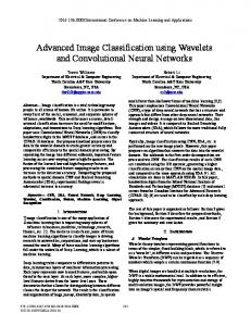
Sigmoid Output LSTM Layer

Max Pooling

Convolutional Layer

Sentence Matrix

when pride comes then comes disgrace

Figure 1: System architecture of the proposed CNNLSTM model.

lowed by a long short-term memory (LSTM) (Hochreiter et al., 1997) layer to form the sentence representation, and a linear regression layer on the top to fit the sentiment intensity of sentences. The details of the CNN, LSTM and their combination are described in the following section.

2

Combining LSTM and CNN for Ordinal Classification

Ordinal classification of sentiment aims at classifying the sentence into ordinal discrete values according to their sentiment intensity. Figure 1 shows the system architecture of the proposed CNNLSTM model for ordinal classification. In the bottom layer, the word vectors of vocabulary words are first trained from a large corpus using word embeddings. For each given sentence, a sentence vector is then built based on the word vectors of words in the sentences, which is further transformed into a matrix representation. The sentence matrix is sequentially passed through a convolutional layer and max pooling layer for multi-point classification. Unlike a conventional LSTM model which directly uses word embeddings as input, the proposed model takes uses outputs from a singlelayer CNN with max pooling. 252

Convolutional Neural Network

In our model, the input of the LSTM layer is an output from the CNN. CNNs have achieved the state-of-the-art results in computer vision applications, and also have been shown to be effective for various NLP applications (Krizhevsky et al., 2012; Kim, 2014; Ma et al., 2015). The CNN architecture used for our tasks is described as follows. Let V denote the vocabulary of words, while d denotes the dimensionality of word vectors, and S ∈ R d ×n denotes the sentence matrix built by concatenating the word vectors occurring in the sentences. Suppose that the sentence T is made up of a sequence of words [d1, d2, …, dn], where n is the length of sentence T. Then the representation of T is given by the matrix S T ∈ R d ×n , where the j-th column corresponds to the embeddings for word dj. Note that for batch processing we the zero-pad sentence matrix ST so that the number of columns is a constant (equal to the max length of sentences) for all sentences in the corpus. We apply a narrow convolution between ST and a filter F ∈ R d ×w of a width w. We then add a bias term and apply a nonlinearity function to obtain a feature map f T ∈ R n − w+1 . The i-th element of f T is given by: f T= [i ] relu (< S T [:, i : i + w − 1], F > +b)

(1)

where S T [:, i : i + w − 1] is the i-to-(i+w-1)-th column of ST and =Trace(A·BT) is the Frobenius inner product. The feature maps are input into a max pooling layer to capture the most salient feature (i.e., the one with the highest value) for a given filter. Filter operation is useful for determining the n-grams, where the size of the n-gram corresponds to the filter length. The above description uses just one filter matrix to generate one feature. In practice, the proposed convolutional layer uses multiple filters in parallel to obtain the feature vectors.

2.2

Recurrent Neural Network

A recurrent neural network (RNN) architecture particularly suited for modelling sequence phenomena (Sak et al., 2014; Zhou et al. 2015). At each time step t, the RNN takes the input vector xt

Name Gold Train Gold Dev Gold Devtest Test

# Tweets released

# Tweets used

# Topics

Avg. Length

6,000

5,346

60

19.49

2,000

1,795

20

19.58

2,000

1,781

20

19.69

20,632

20,632

100

19.62

Name Gold Train Gold Dev Gold Devtest

Here W, U, b are the parameters of an affine transformation and f is an element-wise nonlinearity function. In theory, the RNN can summarize all historical information up to time t with the hidden state ht. In practice, however, a vanilla RNN has difficulty learning long-term dependencies due to the vanishing gradient problem, as the gradient decreases exponentially with the number of network layers and the front layer trains very slowly. Approaches have been developed to deal with vanishing gradient problem, and certain types of RNNs (like LSTM, GRU) are specially designed to get around them. LSTM (Hochreiter et al., 1997) addresses the problem of learning long-term dependencies by augmenting the RNN with a gating mechanism. To illustrate this, the following formulas show how a LSTM calculates a hidden state ht.

it = σ (W i xt + U i ht −1 + bi ) f t = σ (W f xt + U f ht −1 + b f ) ot = σ (W o xt + U o ht −1 + b o ) = gt tanh(W g xt + U g ht −1 + b g )

(3)

= ct f t  ct −1 + it  gt ht = ot  tanh(ct ) Here σ (⋅) and tanh(⋅) are the element-wise sigmoid and hyperbolic tangent functions,  is the element-wise multiplication operator, and it , ft , ot are called the input, forget and output gates respectively. All the gates have the same dimension ds, which is equal to the size of hidden state, and c0, h0 are initialized to zero vectors at t=1. ct is the internal memory of the unit, which could be regarded as 253

# (-1)

# (0)

# (1)

# (2)

87

668

1654

3154

437

43

296

675

933

53

31

233

583

1005

148

Table 2: Distributions of sentiment ratings. # (n) denotes the number of tweets annotated with a rating of n in the range of [-2, -1, ..., 2], corresponding to Strongly Negative, Negative, Negative or Neutral, Positive, Strongly Positive, respectively.

Table 1: Summary of data statistics.

and the hidden state vector ht-1 to produce the next hidden state ht by applying the following recursive operation: (2) ht = f (Wxt + Uht −1 + b)

# (-2)

how we want to combine previous memory and the new input. The gating mechanism allows LSTM to model long-term dependencies. By learning the parameters W j , U j , b j for j ∈{i, f , o, g} , the network learns how its memory cells should behave.

3

Experiments and Evaluation

Dataset. We evaluated the proposed CNN-LSTM model by submitting the results to the SemEval2016 Task 4 subtask. The statistics of the dataset used in this competition are summarized in Table 1. As the original tweets may be removed by Twitter users themselves, we can just download a part of the data in gold training, gold development, and gold development-test dataset. The distribution of sentiment labels shown in Table 2 shows data imbalance. Most of the data were annotated in [-1, 0, 1] labels, and only a few were annotated Very Negative (-2) or Very Positive (2). Implementation details. As mentioned earlier, the proposed method consists of word embeddings and a recurrent convolutional network. Both parts may have their own parameters for optimization. For word embeddings, we used popular pre-trained word vectors from GloVe (Pennington et al., 2014). GloVe is an unsupervised learning algorithm for learning word representation. Training is performed on aggregated global word co-occurrence statistics from a large corpus, and the resulting representation showcases interesting linear substructures in the word vector space. They provide pretrained word vectors trained on 840B tokens from common crawls and have a length of 300. Although the pre-trained word embeddings can capture important semantic and syntactic in-

MAE µ

MAE M

Scores

0.588

1.111

Rank

2

8

Devtest Set

MAE

Table 3: Results of the proposed CNN-LSTM model for SemEval-2016 Task 4 Subtask C.

µ

MAE

Test Set M

MAE µ

MAE M

CNN

0.656

0.992

0.534

0.939

CNNLSTM

0.590

0.974

0.588

1.111

Table 4: Results of CNN-LSTM and CNN alone.

formation of words, they are not sufficient to capture sentiment behaviors in texts. To further improve word embeddings to capture sentiment information, we trained our recurrent convolutional network using an additional dataset from the Vader corpus (Hutto et al., 2014). It contains 4,000 tweets pulled from Twitter’s public timeline, independently annotated by 20 human raters with sentiment ratings in a range of [-4, 4]. We discretized the continuous human-assigned ratings of [-4, 4] to discrete numbers [-2, -1, …, 2] to make them compatible with the task context. The hyper-parameters of the network are chosen based on the performance on the development-test data. We use: rectified linear units (ReLU), filter windows (w) of 3 with 64 feature maps, dropout rate (p) of 0.25, pool length of 2, and mini-bath size of 16. Adagrad update rule is used to automatically tune the learning rate, and micro-averaged MAE is used as the loss function. Early stop mechanism is used to avoid overfitting. The activation function in the top layer is a sigmoid function, which scales each sentiment intensity to the range 0 to 1. These continuous intensity scores are transformed into a five-point scale through the cut-offs: [0, 0.2], (0.2, 0.4], (0.4, 0.6], (0.6, 0.8], (0.8, 1.0] for strongly negative, negative, negative or neutral, positive, strongly positive, respectively. Evaluation metrics. SemEval-2016 Task 4 subtask C published the results for all participants using both macro-averaged mean absolute error ( MAE M ) and micro-averaged mean absolute error ( MAE µ ) (Nakov et al., 2015). The MAE M is defined as: 1 |C | 1 ∑ ∑ | h( X i ) − yi | (4) | C | j 1 | Te j | X i ∈Te j =

= MAE M (h, Te)

where yi denotes the true label of X i , h( X i ) denotes the predicted label, and Te j denotes the set of test documents whose true class is c j . The MAE µ is defined as: 254

= MAE µ (h, Te)

1 ∑ | h( X i ) − yi | | Te | X i ∈Te

(5)

Compared to the micro-averaged MAE µ , the macro-averaged MAE M is more appropriate to measure the classification robustness of systems for imbalanced data. Results. A total of eleven teams participated in subtask C. Table 3 shows the results of the proposed CNN-LSTM model for both MAE µ and MAE M . The proposed method ranked second for MAE µ and eighth for MAE M . The results of MAE µ and MAE M are inconsistent because we used a standard MAE as the loss function for model training and did not consider the imbalanced sentiment labels. Therefore, our model yielded better performance on MAE µ than on MAE M . Table 4 shows the experimental results after the release of test set ratings. We found that the CNNLSTM achieved better performance on the development test set than the test set. Conversely, the CNN alone yielded better performance on the test data than the development-test set.

4

Conclusions

This study presents a deep learning approach to classifying tweets into a five-point scale. The proposed model combines the convolutional neural networks and long short-term memory networks. To better capture the sentiment aspect of words, we further tuned our model using an additional sentiment corpus. Experimental results show that the proposed method archived good performance on the micro-averaged MAE. Future work will focus on exploring more effective features and machine learning methods to improve classification performance for both microand macro-averaged MAE.

Acknowledgments This work was supported by the Ministry of Science and Technology, Taiwan, ROC, under Grant No. NSC102-2221-E-155-029-MY3 and MOST 104-3315-E-155-002.

References Paul Ekman. 1992. An argument for basic emotions. Cognition and Emotion, 6(3-4), 169-200. Alex Go, Richa Bhayani, and Lei Huang. 2009. Twitter sentiment classification using distant supervision. In CS224N Project Report, Stanford. Sepp Hochreiter and Jürgen Schmidhuber. 1997. Long short-term memory. Neural computation, 9(8), 17351780. Xia Hu, Jiliang Tang, Huiji Gao, and Huan Liu. 2013. Unsupervised sentiment analysis with emotional signals. In Proceedings of the 22nd international conference on World Wide Web, pages 607-618. Clayton J. Hutto, and Eric Gilbert. 2014. Vader: A parsimonious rule-based model for sentiment analysis of social media text. In Proceedings of the Eighth International AAAI Conference on Weblogs and Social Media. Yoon Kim. 2014. Convolutional neural networks for sentence classification. In EMNLP, pages 1746–1751, Doha, Qatar. Alex Krizhevsky, Ilya Sutskever, and Geoffrey E. Hinton. 2012. Imagenet classification with deep convolutional neural networks. In Advances in neural information processing systems, pages 1097-1105. B. B. LeCun, John S. Denker, D. Henderson, Richard E. Howard, W. Hubbard, and Lawrence D. Jackel. 1990. Handwritten digit recognition with a backpropagation network. In Advances in neural information processing systems. Fangtao Li, Nathan Liu, Hongwei Jin, Kai Zhao, Qiang Yang, and Xiaoyan Zhu. 2011. Incorporating reviewer and product information for review rating prediction. In Proceedings of the 22nd International Joint Conference on Artificial Intelligence (IJCAI-11), pages 1820-1825. Bing Liu. 2010. Sentiment Analysis and Subjectivity. Handbook of natural language processing, 2, 627666. Mingbo Ma, Liang Huang, Bing Xiang, and Bowen Zhou. 2015. Dependency-based Convolutional Neural Networks for Sentence Embedding. In Proceedings of the 53rd Annual Meeting of the Association for Computational Linguistics (ACL-15), pages 174– 179. Tomas Mikolov, Ilya Sutskever, Kai Chen, Greg S. Corrado, and Jeff Dean. 2013. Distributed representa-

255

tions of words and phrases and their compositionality. In Advances in neural information processing systems, pages 3111-3119. Preslav Nakov, Alan Ritter, Sara Rosenthal, Fabrizio Sebastiani, and Veselin Stoyanov. 2015. Evaluation Measures for the SemEval-2016 Task 4 “Sentiment Analysis in Twitter” (Draft: Version 1.1). Preslav Nakov, Alan Ritter, Sara Rosenthal, Veselin Stoyanov, and Fabrizio Sebastiani. 2016. SemEval2016 Task 4: Sentiment Analysis in Twitter. In Proceedings of the 10th International Workshop on Semantic Evaluation, Association for Computational Linguistics. San Diego, California. Jeffrey Pennington, Richard Socher, and Christopher D. Manning. 2014. Glove: Global Vectors for Word Representation. In Proceedings of the 2014 Conference on Empirical Methods on Natural Language Processing (EMNLP-14), pages 1532-1543. Hasim Sak, Andrew W. Senior, and Françoise Beaufays. 2014. Long short-term memory recurrent neural network architectures for large scale acoustic modeling. In Proceedings of INTERSPEECH-14, pages 338-342. Hassan Saif, Yulan He, Miriam Fernandez, and Harith Alani. 2016. Contextual semantics for sentiment analysis of Twitter. Information Processing & Management, 52(1), 5-19. Maite Taboada, Julian Brooke, Milan Tofiloski, Kimberly Voll, and Manfred Stede. 2011. Lexicon-based methods for sentiment analysis. Computational Linguistics, 37(2):267-307. Hao Wang and Martin Ester. 2014. A sentiment-aligned topic model for product aspect rating prediction. In Proceedings of the 2014 Conference on Empirical Methods in Natural Language Processing (EMNLP14), pages 1192-1202. Jie Zhou and Wei Xu. 2015. End-to-end learning of semantic role labeling using recurrent neural networks. In Proceedings of the 53rd Annual Meeting of the Association for Computational Linguistics (ACL-15), pages 1127–1137. Liang-Chih Yu, Wu, Jheng-Long Wu, Pei-Chann Chang, and Hsuan-Shou Chu. 2013. Using a contextual entropy model to expand emotion words and their intensity for the sentiment classification of stock market news. Knowledge-based Systems. 41:89-97. Liang-Chih Yu, Chung-Hsien Wu, and Fong-Lin Jang. 2009. Psychiatric document retrieval using a discourse-aware model. Artificial Intelligence, 173(7-8): 817-829.