Origin and Evolution of Near-Earth Objects

Morbidelli et al.: Origin and Evolution of Near-Earth Objects

409

Origin and Evolution of Near-Earth Objects A. Morbidelli Observatoire de la Côte d’Azur, Nice, France

W. F. Bottke Jr. Southwest Research Institute, Boulder, Colorado

Ch. Froeschlé Observatoire de la Côte d’Azur, Nice, France

P. Michel Observatoire de la Côte d’Azur, Nice, France

Asteroids and comets on orbits with perihelion distance q < 1.3 AU and aphelion distance Q > 0.983 AU are usually called near-Earth objects (NEOs). It has long been debated whether the NEOs are mostly of asteroidal or cometary origin. With improved knowledge of resonant dynamics, it is now clear that the asteroid belt is capable of supplying most of the observed NEOs. Particular zones in the main belt provide NEOs via powerful and diffusive resonances. Through the numerical integration of a large number of test asteroids in these zones, the possible evolutionary paths of NEOs have been identified and the statistical properties of NEOs dynamics have been quantified. This work has allowed the construction of a steady-state model of the orbital and magnitude distribution of the NEO population, dependent on parameters that are quantified by calibration with the available observations. The model accounts for the existence of ~1000 NEOs with absolute magnitude H < 18 (roughly 1 km in size). These bodies carry a probability of one collision with the Earth every 0.5 m.y. Only 6% of the NEO population should be of Kuiper Belt origin. Finally, it has been generally believed that collisional activity in the main belt, which continuously breaks up large asteroids, injects a large quantity of fresh material into the NEO source regions. In this manner, the NEO population is kept in steady state. The steep size distribution associated with fresh collisonal debris, however, is not observed among the NEO population. This paradox might suggest that Yarkovsky thermal drag, rather than collisional injection, plays the dominant role in delivering material to the NEO source resonances.

1.

INTRODUCTION

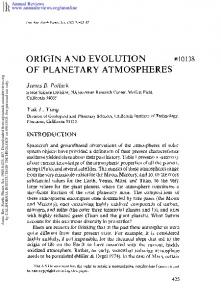
The discovery of 433 Eros in 1898 established the existence of a population of asteroid-like bodies on orbits intersecting those of the inner planets. It was not until the Apollo program in the 1960s and 1970s, however, that lunar craters were shown to be derived from impacts rather than volcanism. With this evidence in hand, it was finally recognized that the Earth-Moon system has been incessantly bombarded by asteroids and comets over the last 4.5 G.y. In 1980, Alvarez et al. presented convincing arguments that the numerous species extinction at the Cretaceous-Tertiary transition were caused by the impact of a massive asteroid (Alvarez et al., 1980). These results brought increasing attention to the objects on Earth-crossing orbits and, more generally, to those having perihelion distances q ≤ 1.3 AU and aphelion distances Q ≥ 0.983 AU. The latter constitute what is usually called the near-Earth-object population (NEOs). Figure 1 shows

the distribution of the known NEOs with respect to their semimajor axis, eccentricity, and inclination. The NEOs are by convention subdivided into Apollos (a ≥ 1.0 AU; q ≤ 1.0167 AU), Atens (a < 1.0 AU; Q ≥ 0.983 AU), and Amors (1.0167 AU < q ≤ 1.3 AU). It is now generally accepted that the NEOs represent a hazard of global catastrophe for human civilization. While the discovery of unknown NEOs is of primary concern, the theoretical understanding of the origin and evolution of NEOs is also of great importance. Together, these efforts can ultimately allow the estimatation of the orbital and size distributions of the NEO population, which in turn makes possible the quantification of the collision hazard and the optimization of NEO search strategies. The purpose of this chapter is to review our current knowledge of these issues. We start in section 2 with a brief historical overview, focused on the many important advances that have contributed to the understanding of the NEO population. In section 3 we discuss how asteroids can escape from the main

409

410

Asteroids III

Apollos

Mars-crossers

Amors

Atens

Main-belt asteroids

40

3:1

5:2

2:1

3:1

5:2

2:1

Inclination

30

20

ν6 10

0

Eccentricity

0.8

0.6

0.4

0.2

ν6 1

1

2

3

Semimajor Axis (AU) Fig. 1. The distribution of NEOs, Mars-crossers and main-belt asteroids with respect to semimajor axis, eccentricity, and inclination. The first 10,000 main-belt asteroids in are shown in gray. The dots represent the Mars-crossers, according to Migliorini et al.’s (1998) definition and identification: bodies with 1.3 < q < 1.8 that intersect the orbit of Mars within the next 300,000 yr. The Amors, Apollos, and Atens are shown as circles, squares, and asterisks respectively. In boldface, the solid curve bounds the Earth-crossing region; the dashed curve delimits the Amor region at q = 1.3 AU, and the dashed vertical line denotes the boundary between the Aten and Apollo populations. The dotted curve corresponds to Tisserand parameter (1) with respect to Jupiter = 3, at i = 0: Jupiter-family comets reside predominantly beyond the curve T = 3. The locations of the 3:1, 5:2, and 2:1 mean motion resonances with Jupiter are shown by vertical dashed lines. The semimajor axis location of the ν6 resonance is roughly independent of the eccentricity but is a function of the inclination: It is shown by the dashed curve on the top panel, while in the bottom panel it is represented for i = 0.

belt and become NEOs, but we also mention the cometary contribution to the NEO population. Section 4 will be devoted to a description of the typical evolutions of NEOs. In these two sections, emphasis will be given to NEO dynamical lifetimes and possible end states. Section 5 will discuss

how the current knowledge on the origin and evolution of NEOs can be utilized to construct a quantitative model of the NEO population. Section 6 will detail the debiased NEO orbital and magnitude distribution resulting from this modeling effort. It will also discuss the implications of this model

Morbidelli et al.: Origin and Evolution of Near-Earth Objects

for the collision probability of NEOs with the Earth, and the collisional and dynamical mechanisms that continuously supply new bodies to the transportation resonances of the asteroid belt. Finally, we discuss open problems and future perspectives in section 7. 2. HISTORICAL OVERVIEW The asteroid vs. comet origin of the NEO population has been debated throughout the last 40 years. With calculations based on a theory of Earth encounter probabilities, Öpik (1961, 1963) claimed that the Mars-crossing asteroid population was not large enough to keep the known Apollo population in steady state. Based on this result, Öpik concluded that about 80% of the Apollos are of cometary origin. The existence of meteor streams associated with some Apollos seemed to provide some support for this hypothesis. Conversely, Anders (1964) proposed that most Apollo objects are small main-belt asteroids that became Earthcrossers as a result of multiple close encounters with Mars. Anders and Arnold (1965) concluded that some Apollos with high eccentricities or inclinations (like 1566 Icarus and 2101 Adonis) might be extinct cometary nuclei, whereas the other Apollos (six known at the time!) should have been of asteroidal origin. Possible asteroidal and cometary sources of Apollo and Amor objects were reviewed in Wetherill (1976). The author considered several mechanisms (including close encounters with Mars, mean motion resonances, and secular resonances) to produce NEOs from the asteroid belt. Ultimately, he concluded that, although qualitatively acceptable, these mechanisms were unable to supply the required number of NEOs by at least an order of magnitude. Thus, Wetherill concluded that most Apollo objects were cores of comets that had lost their volatile material by repeated evaporation. The problem at the time was that resonant dynamics was poorly understood and computation speed was extremely limited. Thus, direct numerical integration of asteroid orbits could not be used to determine the evolutionary paths of NEOs. With the underestimatation of the effect of resonant dynamics, NEO modelers were left with collision as the only viable mechanism for moving asteroids from the main belt directly into the NEO region. The typical ejection velocities of asteroid fragments generated in collisions, however, is ~100 m/s, far too small in most cases to achieve planet-crossing orbits (Wetherill, 1976). The first indication that resonances could force mainbelt bodies to cross the orbits of the planets came from the Ph.D. thesis work of J. G. Williams. In a diagram reported by Wetherill (1979), Williams showed that bodies close to the ν6 resonance have secular eccentricity oscillations with amplitude exceeding 0.25, and therefore they must periodically cross the orbit of Mars. Shortly afterwards, Wisdom (1983, 1985a,b) showed that the 3:1 mean motion resonance has a similar effect: The eccentricity of resonant bodies can have, at irregular time intervals, rapid and large oscillations

411

whose amplitudes exceed 0.3, the threshold value to become a Mars-crosser at the 3:1 location. Following these pioneering works, attention was focused on the 3:1 and ν6 resonances as primary sources of NEOs from the asteroid belt. The dynamical structure of the 3:1 resonance was further explored by Yoshikawa (1989, 1990), Henrard and Caranicolas (1990), and Ferraz-Mello and Klafke (1991) in the framework of the three-body problem. In a more realistic multiplanet solar system model, numerical integrations by Farinella et al. (1993) showed that in the 3:1 resonance the eccentricity evolves much more chaotically than in the three-body problem — a phenomenon later explained by Moons and Morbidelli (1995) — and typically it reaches not only Mars-, but also Earth- and Venus-crossing values (see Moons, 1997, for a review). Concerning the ν6 resonance, the first quantitative numerical results were obtained by Froeschlé and Scholl (1987), who confirmed the role that this resonance has in increasing asteroid eccentricities to Mars-crossing or Earth-crossing values. A first analytic theory of the dynamics in this resonance was developed by Yoshikawa (1987), and later improved by Morbidelli and Henrard (1991) and Morbidelli (1993) (see Froeschlé and Morbidelli, 1994, for a review). Using these advances, Wetherill (1979, 1985, 1987, 1988) developed Monte Carlo models of the orbital evolution of NEOs coming from the ν6 and 3:1 resonances. In these resonances the dynamics were simulated through simple algorithms designed to mimic the results of analytic theories or direct integrations, while elsewhere reduced to the sole effects of close encounters, calculated using twobody scattering formulae (Öpik, 1976). As the Monte Carlo models were refined over time, the cometary origin hypothesis was progressively abandoned as a potential source of NEOs in the inner solar system. Wetherill hypothesized that the ν6 and 3:1 resonances are continuously resupplied via catastrophic collisions and/or cratering events in the main belt, and that enough material is injected into the resonances to keep the NEO population in steady state. Wetherill’s work was later extended by Rabinowitz (1997a,b), who predicted the existence of 875 NEOs larger than 1 km, in remarkable agreement with current estimates. In the 1990s, the availability of cheap and fast workstations allowed the first direct simulations of the dynamical evolution of test particles, initially placed in the NEO region or in the transport resonances, over million-year timescales. Using a Bulirsch-Stoer integrator, a breakthrough result was obtained by Farinella et al. (1994), who showed that NEOs with a < 2.5 AU can easily collide with the Sun, which limits their typical dynamical lifetime to a few million years. It became thus rapidly evident that Monte Carlo codes do not adequately treat the inherently chaotic behavior of bodies in NEO space (see Dones et al., 1999, for a discussion). The introduction of a new numerical integration code (Levison and Duncan, 1994), which extended a numerical symplectic algorithm proposed by Wisdom and Holman (1991), introduced the possibility of numerically

412

Asteroids III

integrating a much larger number of particles, to quantify the statistical properties of NEO dynamics. The subsequent studies have contributed to our current understanding of the origin, evolution, and orbital distribution of NEOs, reviewed in the next sections. 3.

DYNAMICAL ORIGIN OF NEOs

Asteroids become planet crossers by increasing their orbital eccentricity under the action of a variety of resonant phenomena. It is suitable to separately consider “powerful resonances” and “diffusive resonances.” The former can be effectively distinguished from the latter by the existence of associated gaps in the main-belt asteroid distribution. The most notable resonances in the “powerful” class are the ν6 secular resonance at inner edge of the asteroid belt, and the mean motion resonances with Jupiter 3:1, 5:2, and 2:1 at 2.5, 2.8, and 3.2 AU respectively. Their properties are detailed below. The diffusive resonances are so numerous that they cannot be effectively enumerated. Therefore, we will discuss only their generic dynamical effects. The reader can refer to Nesvorný et al. (2002) for a more technical discussion of the dynamical structure of the main asteroid belt. 3.1. ν 6 Resonance The ν6 secular resonance occurs when the precession frequency of the asteroid’s longitude of perihelion is equal to the sixth secular frequency of the planetary system. The latter can be identified with the mean precession frequency of Saturn’s longitude of perihelion, but it is also relevant in the secular oscillation of the eccentricity of Jupiter (see chapter 7 of Morbidelli, 2002). As shown in the top panel of Fig. 1, the ν6 resonance marks the inner edge of the main belt. The effect of the resonance rapidly decays with the distance from the shown curve. To schematize, we divide the ~0.08-AU-wide neighborhood on the righthand side of the curve into a “powerful region” and a “border region,” roughly of equal size (about 0.04 AU each). In the powerful region the resonance causes a regular but large increase of the eccentricity of the asteroids. As a consequence, the asteroids reach Earth- (or Venus-) crossing orbits, and in several cases they collide with the Sun, with their perihelion distance becoming smaller than the solar radius. The median time required to become an Earthcrosser, starting from a quasicircular orbit, is about 0.5 m.y. Accounting also for the subsequent evolution in the NEO region (discussed in section 4), the median lifetime of bodies initially in the ν6 resonance is 2 m.y., the typical end states being collision with the Sun (80% of the cases) and ejection on hyperbolic orbit (12%) (Gladman et al., 1997). The mean time spent in the NEO region is 6.5 m.y. (Bottke et al., 2002a), and the mean collision probability with Earth, integrated over the lifetime in the Earth-crossing region, is ~10 –2 (Morbidelli and Gladman, 1998).

In the border region, the effect of the ν6 resonance is less powerful, but is still capable of forcing the asteroids to cross the orbit of Mars at the top of the secular oscillation cycle of their eccentricity. To enter the NEO region, these asteroids must evolve under the effect of martian encounters, and the required time increases sharply with the distance from the resonance (Morbidelli and Gladman, 1998). The dynamics in this region are complicated by the dense presence of mean motion resonances with Mars, and we will revisit this in section 3.5. 3.2. 3:1 Resonance The 3:1 mean-motion resonance with Jupiter occurs at ~2.5 AU. Inside the resonance, one can distinguish two regions: a narrow central region where the asteroid eccentricity has regular oscillations that cause them to periodically cross the orbit of Mars, and a larger border region where the evolution of the eccentricity is wildly chaotic and unbounded, so that the bodies can rapidly reach Earth-crossing and even Sun-grazing orbits. Under the effect of martian encounters, bodies in the central region can easily travel to the border region and be rapidly boosted into NEO space (see chapter 11 of Morbidelli, 2002). For a population initially uniformly distributed inside the resonance, the median time required to cross the orbit of the Earth is ~1 m.y., the median lifetime is ~2 m.y., and the typical end states are the collision with the Sun (70%) and the ejection on hyperbolic orbit (28%) (Gladman et al., 1997). The mean time spent in the NEO region is 2.2 m.y. (Bottke et al., 2002a), and the mean collision probability with Earth, integrated over the lifetime in the Earth-crossing region, is 2 × 10 –3 (Morbidelli and Gladman, 1998). 3.3. 5:2 Resonance The 5:2 mean-motion resonance with Jupiter is located at 2.8 AU. The mechanisms that allow the rapid and chaotic eccentricity evolution in the border region of the 3:1 resonance in this case extend to the entire resonance (Moons and Morbidelli, 1995). As a consequence, this resonance is the one that pumps the orbital eccentricities on the shortest timescale. The median time required to reach Earth-crossing orbit is ~0.3 m.y., and the median lifetime is 0.5 m.y. Because the resonance is closer to Jupiter than the previous ones, the ejection on hyperbolic orbit is the most typical end state (92%), while the collision with the Sun accounts only for 8% of the losses (Gladman et al., 1997). The mean time spent in the NEO region is 0.4 m.y. and the mean collision probability with Earth, integrated over the lifetime in the Earth-crossing region, is 2.5 × 10 –4. 3.4. 2:1 Resonance Despite the fact that this resonance, located at 3.28 AU, is associated with a deep gap in the asteroid distribution,

Morbidelli et al.: Origin and Evolution of Near-Earth Objects

there are no mechanisms capable of destabilizing the resonant asteroid motion on the short timescales typical of the other resonances. In fact, the dynamical structure of the 2:1 resonance is very complicated (Nesvorný and Ferraz-Mello, 1997; Moons et al., 1998). At the center of the resonance and at moderate eccentricity, there are large regions where the dynamical lifetime is on the order of the age of the solar system. Some asteroids are presently located in these regions (the so-called Zhongguo group), but it is still not completely understood why their number is so small (see Nesvorný and Ferraz-Mello, 1997, for a discussion on a possible cosmogonic mechanism). The regions close to the borders of the resonance are unstable, but several million years are required before an Earth-crossing orbit can be achieved (Moons et al., 1998). Once in NEO space, the dynamical lifetime is only on the order of 0.1 m.y., because the bodies are rapidly ejected by Jupiter onto hyperbolic orbit. The mean collision probability with the Earth, integrated over the lifetime in the Earth-crossing region, is about 5 × 10 –5. 3.5. Diffusive Resonances In addition to the few wide mean-motion resonances with Jupiter described above, the main belt is densely crossed by hundreds of thin resonances: high-order meanmotion resonances with Jupiter (where the orbital frequencies are in a ratio of large integer numbers), three-body resonances with Jupiter and Saturn (where an integer combination of the orbital frequencies of the asteroid, Jupiter, and Saturn is equal to zero; Murray et al., 1998; Nesvorný and Morbidelli, 1998, 1999), and mean motion resonances with Mars (Morbidelli and Nesvorný, 1999). Because of these resonances, many — if not most — main-belt asteroids are chaotic (see Nesvorný et al., 2002, for discussion). The effect of this chaoticity is very weak. The mean semimajor axis is bounded within the narrow resonant region; the proper eccentricity and inclination (see Knezevic et al., 2002) slowly change with time, in a chaotic diffusion-like process. The time required to reach a planet-crossing orbit (Mars-crossing in the inner belt, Jupiter-crossing in the outer belt) ranges from several 107 yr to billions of years, depending on the resonances and starting eccentricity (Murray and Holman, 1997). Integrating real objects in the inner belt (2 < a < 2.5 AU) for 100 m.y., Morbidelli and Nesvorný (1999) estimated that chaotic diffusion drives about two asteroids larger than 5 km into the Mars-crossing region every million years. The escape rate is particularly high in the region adjacent to the ν6 resonance, because of the effect of the latter, but also because of the dense presence of mean motion resonances with Mars. The high rate of diffusion of asteroids from the inner belt can explain the existence of the conspicuous population of Mars-crossers. Following Migliorini et al. (1998), we define the latter as the population of bodies with q > 1.3 AU that intersect the orbit of Mars within a secular

413

cycle of their eccentricity oscillation (in practice within the next 300,000 yr). The Mars-crossers are about 4× more numerous than the NEOs of equal absolute magnitude (statistics done on bodies with H < 15, which constitute an almost complete sample in both populations). It was believed in the past that most q > 1.3 AU Mars-crossers were bodies extracted from the main transportation resonances (i.e., 3:1 and ν6 resonances) by close encounters with Mars. But, as pointed out by Migliorini et al., the eccentricity of bodies in these resonances increases so rapidly to Earthcrossing values that only a few bodies can be extracted by Mars and emplaced in the Mars-crossing region with q > 1.3 AU. This low probability is only partially compensated by the fact that, once bodies enter this Mars-crossing region, their dynamical lifetime becomes about 10× longer. Indeed, work on numerical integrations indicate that if the 3:1 and ν6 resonances sustained both the Mars-crossing population with q > 1.3 AU and the NEO population, the ratio between these populations would be only 0.25 (i.e., 16× smaller than observed). Figure 1 shows that the population of Mars-crossers extends up to a ~ 2.8 AU, suggesting that the phenomenon of chaotic diffusion from the main belt extends at least up to this threshold. The (a,i) panel shows that in addition to the main population situated below the ν6 resonance (called IMC hereafter), there are two groups of Mars-crossers with orbital elements that mimic those of the Hungaria (1.77 < a < 2.06 AU and i > 15°) and Phocaea (2.1 < a < 2.5 AU and i >18°) populations, arguing for the effectiveness of chaotic diffusion as well in these high-inclination regions. To reach Earth-crossing orbit, the Mars-crossers random walk in semimajor axis under the effect of martian encounters until they enter a resonance that is strong enough to further decrease their perihelion distance below 1.3 AU. For the IMC group, the median time required to become an Earth-crosser is ~60 m.y.; about two bodies larger than 5 km become NEOs every million years (Michel et al., 2000b), consistent with the supply rate from the main belt estimated by Morbidelli and Nesvorný (1999). The mean time spent in the NEO region is 3.75 m.y. (Bottke et al., 2002a). The median time to reach Earth-crossing orbits from the two groups of high inclined Mars-crossers exceeds 100 m.y. (Michel et al., 2000b). The paucity of Mars-crossers with a > 2.8 AU is not due to the inefficiency of chaotic diffusion in the outer asteroid belt. It is simply the consequence of the fact that the dynamical lifetime of bodies in the Mars-crossing region drops with increasing semimajor axis toward the Jupiter-crossing limit. In addition, the observational biases for kilometersized asteroids are more severe than in the a < 2.8 AU region. In fact, the outer belt is densely crossed by high-order mean-motion resonances with Jupiter and three-body resonances with Jupiter and Saturn, so an important escape rate into the NEO region should be expected. Bottke et al. (2002a) have integrated for 100 m.y. nearly 2000 observed main-belt asteroids with 2.8 < a < 3.5 AU and i < 15° and

414

Asteroids III

q < 2.6 AU; almost 20% of them entered the NEO region. About 30,000 bodies with H < 18 can be estimated to exist in the region covered by Bottke et al.’s initial conditions. According to Bottke et al. integrations, in a steady-state scenario this population could provide ~600 new H < 18 NEOs per million years, but the mean time that these bodies spend in the NEO region is only ~0.15 m.y. 3.6. Cometary Contribution Despite the fact that asteroids dominate the NEO population with small semimajor axes, comets are also expected to be important contributors to the overall NEO population. Comets can be subdivided into two groups: those coming from the Kuiper Belt (or, more likely, the scattered disk) and those coming from the Oort Cloud. The first group includes the Jupiter-family comets (JFCs). Their orbital distribution has been well-characterized with numerical integrations by Levison and Duncan (1997). Their cometary test bodies, however, remained confined to a > 2.5 AU orbits, probably because terrestrial planet perturbations and nongravitational forces were not included in the simulations. The population of comets of Oort Cloud origin includes the long periodic and Halley-type groups. To explain the orbital distribution of the observed population, several researchers have postulated that the comets from the Oort Cloud rapidly “fade” away, either becoming inactive or splitting into small components (Wiegert and Tremaine, 1999; Levison et al., 2001). Since the number of faded comets to new comets has yet to be determined, calculating the population on NEO orbits is problematic. Despite this, best-guess estimates suggest that impacts from Oort Cloud comets may be responsible for 10–30% of the craters on Earth (see Weissman et al., 2002). However, recent unpublished work (Levison et al., personal communication, 2001) reduces this estimate to only ~1%. 4.

EVOLUTION IN NEO SPACE

The dynamics of the bodies in NEO space is strongly influenced by close encounters with the planets. Each encounter provides an impulse velocity to the body’s trajectory, causing the semimajor axis to “jump” by a quantity depending on the geometry of the encounter and the mass of the planet. The change in semimajor axis is correlated with the change in eccentricity (and inclination) by the quasiconservation of the so-called Tisserand parameter T=

ap a

+2

a 1 − e2 cos i ap

(1)

relative to the encountered planet with semimajor axis ap (Öpik, 1976). An encounter with Jupiter can easily eject the body from the solar system (a = ∞ or negative), while this is virtually impossible in encounters with the terrestrial planets.

Under the sole effect of close encounters with a unique planet, and neglecting the effects on the inclination, a body would randomly walk on a curve of the (a, e) plane defined by T = constant. These curves are transverse to all meanmotion resonances and to most secular resonances, so that the body can be extracted from a resonance and be transported into another one. Resonances, on the other hand, change the eccentricity and/or the inclination of the bodies, keeping the semimajor axis constant. The real dynamics in the NEO region are therefore the result of a complicated interplay between resonant dynamics and close encounters (see Michel et al., 1996a). A further complication is that encounters with several planets can occur at the same time, thus breaking the Tisserand parameter approximation even in the absence of resonant effects. As anticipated in the previous section, most bodies that become NEOs with a > 2.5 AU are preferentially transported to the outer solar system or are ejected on hyperbolic orbit. In fact, if the eccentricity is sufficiently large, the NEOs in this region approach the Jupiter-crossing limit where the giant planet can scatter them outward. At that point, their dynamics become similar to that of Jupiter-family comets. A typical example is given by the rightmost evolution in Fig. 2a. The body penetrates the NEO region by increasing its orbital eccentricity inside the 5:2 resonance until e ~ 0.7; the encounters with Jupiter then extract it from the resonance and transport it to a larger semimajor axis. Only bodies extracted from the resonance by Mars or Earth and rapidly transported on a low-eccentricity path to a smaller semimajor axis could escape the scattering action of Jupiter. But this evolution is increasingly unlikely as the initial semimajor axis is set to larger and larger values. Conversely, the bodies on orbits with a ~ 2.5 AU or smaller do not approach Jupiter even at e ~ 1, so that they end their evolution preferentially by impacting the Sun. Most of the bodies originally in the 3:1 resonance are transported to e ~ 1 without having a chance of being extracted from the resonance. For the bodies originally in the ν6 resonance, a temporary extraction from the resonance in the Earth-crossing space is more likely (Fig. 2a). Most of the IMCs with 2 < a < 2.5 AU eventually enter the 3:1 or the ν6 resonance and subsequently behave as resonant particles. Figures 2b and 2c show evolutionary paths from ν6 and 3:1, which are unlikely (they occur in ~10% of the cases), but extremely important to understanding the observed NEO orbital distribution. In these cases, encounters with Earth or Venus extract the body from its original resonance and transport it into the region with a < 2 AU (hereafter called the “evolved region”). Once in the evolved region, the dynamical lifetime grows longer (~10 m.y., Gladman et al., 2000) because there are no statistically significant dynamical mechanisms that pump the eccentricity up to Sun-grazing values. To be dynamically eliminated, the bodies in the evolved region must either collide with a terrestrial planet (rare) or be driven back to a > 2 AU, where powerful resonances can push them into the Sun. The enhanced lifetime partially compensates for the difficulty these

Morbidelli et al.: Origin and Evolution of Near-Earth Objects

415

1

(a) Eccentricity

0.8 0.6 0.4 0.2

ν6

0

1

1.5

3:1

2

5:2

2.5

3

2.5

3

1

(b) Eccentricity

0.8 0.6 0.4 0.2 ν6 0

1

1.5

2

1

(c) Eccentricity

0.8 0.6 0.4 0.2 0

3:1 1

2

2.5

Semimajor Axis (AU)

Fig. 2. Orbital evolutions of objects leaving the main asteroid belt. The curves indicate the sets of orbits having aphelion or perihelion at the semimajor axis of one of the planets Venus, Earth, Mars, or Jupiter. (a) Common evolution paths from the ν6, 3:1, and 5:2 resonances. (b) A long-lived particle from the ν6 resonance. The evolution before 20 m.y. is shown in black, and the subsequent one is illustrated in gray. (c) A long-lived particle from 3:1; black dots show the evolutions during the first 15 m.y. Adapted from Gladman et al. (1997).

objects have in reaching the evolved region. Thus, the latter should host 38% and 70% respectively of all NEOs of 3:1 and ν6 origin (Bottke et al., 2002a). The dynamical evolution in the evolved region can be very tortuous, and does not follow any clear curve of constant Tisserand parameter. The main reason is that first-order secular resonances are present and effective in this region, and continuously change the perihelion distance of the body (see Michel et al., 1996b; Michel and Froeschlé, 1997; Michel, 1997a). In some cases the perihelion distance can be temporarily raised above 1 AU, where, in the absence of encounters with Earth, the body can reside for several million years (notice the density of points at a ~ 1.62, e ~ 0.3 in Fig. 2b). The Kozai resonance (Michel and Thomas,

1996; Gronchi and Milani, 1999) and the mean-motion resonances with the terrestrial planets (Milani and Baccili, 1998) can also provide a protection mechanism against close approaches, thus stabilizing the motion of the bodies temporarily locked into them. Among mean-motion resonance trapping, of importance is the temporary capture in a coorbital state, where the body follows horseshoe and/or tadpole librations about a planet. This phenomenon has been observed in the numerical simulations by Michel et al. (1996b), Michel (1997b), and Christou (2000), and a detailed theory has been developed by Namouni (1999). The asteroid (3753) 1986 T0 has been shown to currently evolve on a highly inclined horseshoe orbit around Earth (Wiegert et al., 1997).

416

Asteroids III

We point out a few additional features in the evolution of Fig. 2b that we find remarkable. The body passes into the region with a ~ 1 AU and e < 0.1 twice, where the socalled small Earth approachers (SEAs) have been observed (Rabinowitz et al., 1993). This shows that the SEAs could come from the main belt. Also, the evolution penetrates in the region inside Earth’s orbit (aphelion distance smaller than 0.983 AU). It is then plausible to conjecture the existence of a population of “interior to the Earth objects” (IEOs), despite the fact that observations have not yet discovered any such bodies (Michel et al., 2000a). 5. QUANTITATIVE MODELING OF THE NEO POPULATION The observed orbital distribution of NEOs is not representative of the real distribution, because strong biases exist against the discovery of objects on some types of orbits. Given the pointing history of a NEO survey, the observational bias for a body with a given orbit and absolute magnitude can be computed as the probability of being in the field of view of the survey, with an apparent magnitude brighter than the limit of detection (see Jedicke et al., 2002). Assuming random angular orbital elements of NEOs, the bias is a function B(a, e, i, H), dependent on semimajor axis, eccentricity, inclination, and absolute magnitude H. Each NEO survey has its own bias. Once the bias is known, in principle the real number of objects N can be estimated as N(a, e, i, H) = n(a, e, i, H)/B(a, e, i, H) where n is the number of objects detected by the survey. The problem, however, is resolution; even a coarse binning in the four-dimensional orbital-magnitude space of the bias function and the observed distribution requires the use of about 10,000 cells. The total number of NEOs detected by the most efficient surveys is a few hundreds. Thus n is zero on the vast majority of the cells, and it is equal to 1 in most other cells; cells with n > 1 are very rare. The debiasing of the NEO population is therefore severely affected by small number statistics. To circumvent this problem, one can consider projected distributions of the detected NEOs, such as n(a, e), n(i), and n(H), and try to debias each of them independently, using a mean bias [B(a, e), B(i), or B(H)], computed by summation of B(a, e, i, H) over the hidden dimensions (Stuart, 2000). However, the study of the dynamics shows that the inclination distribution is strongly dependent on a and e: Dynamically young NEOs with large semimajor axes roughly preserve their main-belt-like inclination, while dynamically old NEOs in the evolved region have a much broader inclination distribution, due to the action of the multitude of resonances that they crossed during their lifetime. As a consequence, this simplified debiasing method can lead to very approximate results. An alternative way to construct a model of the real distribution of NEOs heavily relies on the dynamics. In fact, from numerical integrations, it is possible to estimate the steady-state orbital distribution of the NEOs coming from

each of the main source regions defined in section 3 (see below for the method). In this approach, the key assumption is that the NEO population is currently in steady state. This requires some comments. The analysis of lunar and terrestrial craters suggests that the impact flux on the EarthMoon system has been more or less constant for the last ~3 G.y. (Grieve and Shoemaker, 1994), thus supporting the idea of a gross steady state of the NEO population. This view is challenged, however, by the analysis of the asteroid belt, which shows that the formation of several asteroid families occurred over the age of the solar system (see Zappalà et al., 2002). The formation of asteroid families may have had two consequences on the time evolution of the NEO population: 1. A large number of asteroids might have been injected into the resonances at the moment of the parent bodies breakup, producing a temporary large increase in the NEO population (Zappalà et al., 1997). Because the median lifetime of resonant particles is ~2 m.y., the NEO population should have returned to a normal “steady-state” value in about 10 m.y. Being short-lived, these temporary spikes in the total number of NEOs should not have left an easily detectable trace in the terrestrial planet crater record. However, evidence that one of these spikes really happened — at least for meteorite-sized NEOs — comes from the discovery of 17 “fossil meteorites” in a 480-m.y.-old limestone (Schmitz et al., 1996, 1997). These discoveries suggest that the influx of meteorites during that 1–2-m.y. period was 10– 100× higher than at present. If the general belief that families are several 108–109 yr old (Marzari et al., 1995) is correct, the current NEO population should not be affected by any of these hypothetical spikes. 2. The rate at which bodies have been continuously supplied to some transporting resonance(s) might have increased after a major family formation event enhanced the population in the resonance vicinity. In this case the NEO population would have evolved to a new and different steady-state situation. Possible evidence for such a transition comes from Culler et al. (2000), who claimed that the lunar impactor flux has been higher by a factor of 3.7 ± 1.2 over the last 400 m.y. than over the previous 3 G.y. Even this case, however, would not invalidate the steady-state assumption, essential for constructing a model of the NEO distribution based on statistics of the orbital dynamics. In fact, being short-lived, the NEO population preserves no memory of what happened several 108 yr ago; what is important is that the NEO population has been in the same “steady state” during the last several ~107 yr, namely on a timescale significantly longer than the mean lifetime in the NEO region. The recipe to compute the steady-state orbital distribution of the NEOs for a given source is as follows. First, the dynamical evolutions of a statistically significant number of particles, initially placed in the NEO source region(s), are numerically integrated. The particles that enter the NEO region are followed through a network of cells in the (a, e, i) space during their entire dynamical lifetime. The mean time spent in each cell (called residence time hereafter) is com-

Morbidelli et al.: Origin and Evolution of Near-Earth Objects

puted. The resultant residence time distribution shows where the bodies from the source statistically spend their time in the NEO region. As is well known in statistical mechanics, in a steady-state scenario, the residence time distribution is equal to the relative orbital distribution of the NEOs that originated from the source. This dynamical approach was first introduced by Wetherill (1979) and was later imitated by Rabinowitz (1997a). Unfortunately, these works used Monte Carlo simulations, which allowed only a very approximate knowledge of the statistical properties of the dynamics. Bottke et al. (2000) have reactualized the approach using modern numerical integrations. They computed the steady-state orbital distributions of the NEOs from three sources: the ν6 resonance, the 3:1 resonance, and the IMC population. The latter was considered to be representative of the outcome of all diffusive resonances in the main belt up to a = 2.8 AU. The overall NEO orbital distribution was then constructed as a linear combination of these three distributions, thus obtaining a two-parameter model. The NEO magnitude distribution, assumed to be source-independent, was constructed so its shape could be manipulated using an additional parameter. Combining the resulting NEO orbitalmagnitude distribution with the observational biases associated with the Spacewatch survey (Jedicke, 1996), Bottke et al. (2000) obtained a model distribution which could be fit to the orbits and magnitudes of the NEOs discovered or accidentally rediscovered by Spacewatch. To have a better match with the observed population at large a, Bottke et al. (2002a) extended the model by also considering the steadystate orbital distributions of the NEOs coming from the outer asteroid belt (a > 2.8 AU) and from the Transneptunian region. The resulting best-fit model nicely matches the distribution of the NEOs observed by Spacewatch, without restriction on the semimajor axis (see Fig. 10 of Bottke et al., 2002a). Notice that, once the values of the parameters of the model are computed by best-fitting the observations of one survey, the steady-state orbital-magnitude distribution of the entire NEO population is determined. This distribution is valid also in those regions of the orbital space that have never been sampled by any survey because of extreme observational biases. For instance, Bottke et al. models predict the total number of IEOs, despite the fact that none of these objects has ever been detected. This underlines the power of the dynamical approach for debiasing the NEO population. 6. DEBIASED NEO POPULATION This section is based strongly on the results of the modeling effort by Bottke et al. (2002a). Unless explicitly stated, all numbers reported below are taken from that work. The total NEO population contains 960 ± 120 objects with absolute magnitude H < 18 (roughly 1 km in diameter) and a < 7.4 AU. The observational completeness of this population as of July 2001 is ~45%. The NEO absolute magnitude distribution is of type N( 16, e > 0.4, a = 1–3 AU, and i = 5°–40°. Overall, 32 ± 1% of the NEOs are Amors, 62 ± 1% are Apollos, and 6 ± 1% are Atens. Of the NEOs, 49 ± 4% should be in the evolved region (a < 2 AU), where the dynamical lifetime is strongly enhanced. The ratio between the IEO and the NEO populations is about 2%. With this orbital distribution, and assuming random values for the argument of perihelion and the longitude of node, about 21% of the NEOs turn out to have a minimal orbital intersection distance (MOID) with the Earth smaller than 0.05. The MOID is defined as the minimal distance between the osculating orbits of two objects. NEOs with MOID < 0.05 AU are classified as potentially hazardous objects (PHOs), and the accurate orbital determination of these bodies is considered a top priority. To estimate the collision probability with the Earth, we use the collision probability model described by Bottke et al. (1994). This model, which is an updated version of similar models described by Öpik (1951), Wetherill (1967), and Greenberg (1982), assumes that the values of the mean anomalies of the Earth and the NEOs are random. The gravitational attraction exerted by the Earth is also included. We find that, on average, the Earth collides with an H < 18 NEO once every 0.5 m.y. Figure 4 shows how the collision probability is distributed as a function of the NEO orbital elements or, equivalently, which NEOs carry most of the collisional hazard. For an individual object, the collision probability with the Earth decreases with increasing semimajor axis, eccentricity, and/or inclination (Morbidelli and Gladman, 1998). For this reason, the histograms in Fig. 4 are very different from those in Fig. 3: The a distribution peaks at 1 AU instead of 2.2 AU, the e distribution is more symmetric with respect to the e = 0.5 value, and the i distribution is much steeper. The stated goal of the Spaceguard survey, a NEO survey program proposed in the early 1990s, was to discover 90% of the NEOs with H < 18 (Morrison, 1992). However, it would be more appropriate to state the goal in terms of discovering the NEOs carrying 90% of the total collision probability. Figures 3 and 4 show that the two goals are not equivalent. For instance, the Atens, even though they are only 6% of the total NEO population, carry about 20% of the total collision probability; thus, their discovery (of sec-

418

Asteroids III

100 60

Number

Number

80 40

60

40 20 20 0

0

1

2

3

4

0 0.0

5

0.2

Semimajor Axis a (AU)

0.4

0.6

0.8

1.0

17

18

Eccentricity e

300 250

Number

Number

150

100

200 150 100

50

50 0

0

20

40

60

80

Inclination i (degrees)

0 13

14

15

16

Absolute Magnitude H

Fig. 3. The steady-state orbital and absolute magnitude distribution of NEOs for H < 18. The predicted NEO distribution (solid line) is normalized to 960 objects. It is compared with the 426 known NEOs for all surveys (shaded histogram). From Bottke et al. (2002a).

ondary importance for the original Spaceguard goal) becomes a top priority, when collisional hazards are taken into account. By applying the same collision probability calculations to the H < 18 NEOs discovered so far, we find that the known objects carry about 47% of the total collisional hazard. Thus, the current completeness of the population computed in terms of collision probability is about the same of that computed in terms of number of objects. This seems to imply that the current surveys discover NEOs more or less evenly with respect to the collision probability with the Earth. In Fig. 4 the shaded histogram shows how the collision probability of the known NEOs is distributed as a function of the orbital elements. Finally, we discuss the origin of NEOs. The Bottke et al. (2002a) model implies that 37 ± 8% of the NEOs with 13 < H < 22 come from the ν6 resonance, 25 ± 3% from the IMC population, 23 ± 9% from the 3:1 resonance, 8 ± 1% from the outer-belt population, and 6 ± 4% from the Transneptunian region. Thus, the long-debated cometary contribution to the NEO population probably does not ex-

ceed 10%. Note, however, that the Bottke et al. model does not account for the contribution of comets of Oort Cloud origin, which is still largely unconstrained for the reasons explained in section 3.6. These comets should be relegated to orbits with a > 2.6 AU and/or orbits with large eccentricities and inclinations. About 800 bodies with H < 18, 70% of which come from the outer main belt, should escape from the asteroid belt every million years in order to sustain the NEO population. These fluxes may seem huge, but they only imply a mass loss of ~5 × 1016 kg/m.y., or the equivalent of 6% of the total mass of the asteroid belt over 3.5 G.y. (assuming that the flux has been constant over this timescale). By itself, this flux does not constrain the mechanism (or mechanisms) that resupply the transporting (powerful and diffusing) resonances with new bodies. The shallow size distribution of NEOs, however, suggests that collisional injection probably does not play a dominant role in the delivery of asteroidal material to resonances. If it did, the NEOs, being fragments from catastrophic breakups, would have a much steeper size distribution, at least like that of

Morbidelli et al.: Origin and Evolution of Near-Earth Objects

419

Number of Collisions/100 m.y.

Number of Collisions/100 m.y.

20 12 10 8 6 4 2 0

0

1

2

4

3

15

10

5

0 0.0

Number of Collisions/100 m.y.

Semimajor Axis a (AU)

0.2

0.4

0.6

0.8

1.0

Eccentricity e

50 40 30 20 10 0

0

20

40

60

80

Inclination i (degrees) Fig. 4. Number of Earth impacts with H < 18 NEOs as a function of the NEO orbital distribution. The solid histogram shows the expected distribution, deduced from the Bottke et al. (2002a) model; the shaded histogram is obtained applying the collision probability calculation to the population of known objects.

the observed asteroid families (Tanga et al., 1999; Campo Bagatin et al., 2000). Recall that the mean lifetime in the NEO region is only a few million years, too short for collisional erosion to significantly reduce the slope of a size distribution dominated by fresh debris (bodies with a diameter of about 170 m have a collisional lifetime >100 m.y.; Bottke et al., 1994). Moreover, it is unclear how collisional injection could explain the relative abundance of multikilometer objects in the NEO population. According to standard collision models, only the largest (and most infrequent) catastrophic disruption events are capable of throwing multikilometer objects into the transporting major resonances (Menichella et al., 1996; Zappalà and Cellino, 2002). The NEO size distribution shows some interesting similarities with the main-belt size distribution. At present, a direct estimate of the latter is available only for D > 2 km asteroids (Jedicke and Metcalfe, 1998), but its shape has been extrapolated to smaller sizes by Durda et al. (1998) using a collisional model. The results suggest the main belt’s size distribution for 0.2 < D < 5 km asteroids is NEOlike or possibly shallower. The results of recent surveys

(Ivezic et al., 2001; Yoshida et al., 2001) seem to confirm this expectation. Although more quantitative studies are needed for a definite conclusion, we suspect that this paradox might be solved by the Yarkovsky effect. The latter forces kilometersized bodies to drift in semimajor axis by ~10 –4 AU m.y.–1 (Farinella and Vokrouhlický, 1999; see also Bottke et al., 2002b), enough to bring into resonance a large — possibly sufficient — number of bodies. The Yarkovsky drift rate is slow enough that the size distribution of fresh collisional debris would have the time to collisionally evolve to a shallower, main-belt-like slope. 7.

CONCLUSIONS AND PERSPECTIVES

The massive use of long-term numerical integrations have boosted our understanding of the origin, evolution, and steady-state orbital distribution of NEOs. The “powerful resonances” of the main belt have been shown to transport the asteroids into the NEO region on a timescale of only a few 105 yr. On the other hand, we now understand that these

420

Asteroids III

resonances eliminate most of these same bodies by forcing them to collide with the Sun. The “diffusive resonances” have been shown to be additional important sources of NEOs. The steady-state orbital distributions of the NEO subpopulations related to the various sources have been computed. This work has allowed the construction of a quantitative model of the debiased orbital and magnitude distribution of the NEO population, calibrated on available observations. Despite the steady progress, the current understanding of the NEO population is still lacking in several areas. As more and more NEOs are continuously found, the NEO model presented here will certainly need to be refined. Moreover, although it is now clear that the vast majority of NEOs with semimajor axes inside Jupiter’s orbit are of asteroidal origin, the contribution of inactive comets coming from the Oort Cloud remains poorly quantified. The most unclear part of the scenario regarding the origin and evolution of NEOs concerns the mechanisms that resupply the transporting resonances with new asteroids. At the end of the previous section, we discussed several arguments that suggest that the Yarkovsky effect plays the dominant role in moving small asteroids to powerful and diffusive resonances. More definitive conclusions, however, will require a better knowledge of the orbital and size distribution of the main-belt population in the kilometer size range, in order to quantify the availability of material in the neighborhood of the transporting resonances. Our understanding of asteroidal and cometary collisional physics is also limited, and additional work will be needed to determine more accurately the size-frequency and velocity-frequency distributions of asteroid disruption events. Simulations are also required to understand the interaction of the Yarkovskydrifting bodies with the multitude of diffusive resonances that they encounter. It is possible that small bodies drift too fast to be efficiently captured by these thin resonances. If it turns out that different mechanisms resupply different NEO source regions, it may be inappropriate to assume that the NEO subpopulations coming from the various sources described in this chapter have the same size distribution. Finally, we need to better understand the changes that occurred over the last 3.8 G.y. (after the so-called late heavy bombardment), in terms of the total number of NEOs and their size or orbital distribution. For this purpose, we need to understand whether the members of asteroid families dominate the rest of the main-belt asteroid population. If they do (as claimed by Zappalà and Cellino, 1996), the formation of new families should have significantly changed the main-belt population and consequently altered the feeding rate of the NEO population. If not, the breakup of asteroid families can be considered noise in the history of the NEO population. We believe that a detailed knowledge of the physical properties of asteroids close to the transporting resonances will eventually allow us to indirectly but accurately deduce the compositional distribution of the NEO population. In turn, this will enable the conversion of NEO absolute mag-

nitudes into diameters, and better quantify the collisional hazard (frequency of collisions as a function of the impact energy) for Earth. REFERENCES Alvarez L. W., Alvarez W., Asaro F., and Michel H. V. (1980) Extraterrestrial cause for the Cretaceous Tertiary extinction. Science, 208, 1095–1099. Anders E. (1964) Origin, age and composition of meteorites. Space Sci. Rev., 3, 583–574. Anders E. and Arnold J. R. (1965) Age of craters on Mars. Science, 149, 1494–1496. Bottke W. F., Nolan M. C., Greenberg R., and Kolvoord R. A. (1994) Velocity distributions among colliding asteroids. Icarus, 107, 255–268. Bottke W. F., Jedicke R., Morbidelli A., Petit J. M., and Gladman B. (2000) Understanding the distribution of near-Earth asteroids. Science, 288, 2190–2194. Bottke W. F., Morbidelli A., Jedicke R., Petit J. M., Levison H. F., Michel P., and Metcalfe T. S. (2002a) Debiased orbital and size distribution of the Near Earth Objects. Icarus, in press. Bottke W. F. Jr., Vokrouhlický D., Rubincam D. P., and Broz M. (2002b) Dynamical evolution of asteroids and meteoroids using the Yarkovsky effect. In Asteroids III (W. F. Bottke Jr. et al., eds.), this volume. Univ. of Arizona, Tucson. Campo Bagatin A., Martinez V. J., and Paredes S. (2000) Multinomial fits to the observed main belt asteroid distribution (abstract). In Bull. Am. Astron. Soc., 32, 813. Christou A. (2000) A numerical survey of transient co-orbitals of the terrestrial planets. Icarus, 144, 1–20. Culler T. S., Becker T. A., Muller R. A., and Renne P. R. (2000) Lunar impact history from 40Ar/39Ar dating of glass spherules. Science, 287, 1785–1788. Dones L., Gladman B., Melosh H. J., Tonks W. B., Levison H. F., and Duncan M. (1999) Dynamical lifetimes and final fates of small bodies: Orbit integrations vs Öpik calculations. Icarus, 142, 509–524. Durda D. D., Greenberg R., and Jedicke R. (1998) Collisional models and scaling laws: A new interpretation of the shape of the main-belt asteroid size distribution. Icarus, 135, 431– 440. Farinella P. and Vokrouhlický D. (1999) Semimajor axis mobility of asteroidal fragments. Science, 283, 1507–1510. Farinella P., Froeschlé Ch., and Gonczi R. (1993). Meteorites from the asteroid 6 Hebe. Cel. Mech. Dyn. Astron., 62, 87–305. Farinella P., Froeschlé Ch., Gonczi R., Hahn G., Morbidelli A., and Valsecchi G. B. (1994) Asteroids falling onto the Sun. Nature, 371, 315–317. Ferraz-Mello S. and Klafke J. C. (1991) A model for the study of the very high eccentricity asteroidal motion: The 3:1 resonance. In Predictability, Stability and Chaos in N-Body Dynamical Systems (A. E. Roy, ed.), pp. 177–187. Plenum, New York. Froeschlé Ch. and Morbidelli A. (1994) The secular resonances in the solar system. In Asteroids, Comets, and Meteors, 1993 (A. Milani et al., eds.), pp. 189–204. Kluwer, Boston. Froeschlé Ch. and Scholl H. (1987) Orbital evolution of asteroids near the secular resonance ν6. Astron. Astrophys., 179, 294–303. Gladman B., Migliorini F., Morbidelli A., Zappalà V., Michel P., Cellino A., Froeschlé Ch., Levison H., Bailey M., and Duncan

Morbidelli et al.: Origin and Evolution of Near-Earth Objects

M. (1997) Dynamical lifetimes of objects injected into asteroid belt resonances. Science, 277, 197–201. Gladman B., Michel P., and Froeschlé Ch. (2000) The Near-Earth Object population. Icarus, 146, 176–189. Greenberg R. (1982) Orbital interactions — A new geometrical formalism. Astron. J., 87, 184–195. Grieve R. A. and Shoemaker E. M. (1994) The record of past impacts on Earth. In Hazards Due to Comets and Asteroids (T. Gehrels and M. S. Matthews, eds.), pp. 417–462. Univ. of Arizona, Tucson. Gronchi G. F. and Milani A. (1999) The stable Kozai state for asteroids and comets with arbitrary semimajor axis and inclination. Astron. Astrophys., 341, 928–937. Henrard J. and Caranicolas N. D. (1990) Motion near the 3:1 resonance of the planar elliptic restricted three body problem. Cel. Mech. Dyn. Astron., 47, 99–108. Ivanov B. A., Neukum G., Hartmann W. K., and Bottke W. F. Jr. (2002) Comparison of size-frequency distributions of impact craters and asteroids and the planetary cratering rate. In Asteroids III (W. F. Bottke Jr. et al., eds.), this volume. Univ. of Arizona, Tucson. Ivezic Z. and 31 colleagues (2001) Solar system objects observed in the Sloan digital sky survey commissioning data. Astron. J., 122, 2749–2784. Jedicke R. (1996) Detection of near Earth asteroids based upon their rates of motion. Astron. J., 111, 970–983. Jedicke R. and Metcalfe T. S. (1998) The orbital and absolute magnitude distributions of main belt asteroids. Icarus, 131, 245–260. Jedicke R., Larsen J., and Spahr T. (2002) Observational selection effects in asteroid surveys and estimates of asteroid population sizes. In Asteroids III (W. F. Bottke Jr. et al., eds.), this volume. Univ. of Arizona, Tucson. Knezevic Z., Lemaitre A., and Milani A. (2002) Asteroid proper elements determination. In Asteroids III (W. F. Bottke Jr. et al., eds.), this volume. Univ. of Arizona, Tucson. Levison H. F. and Duncan M. J. (1994) The long-term dynamical behavior of short-period comets. Icarus, 108, 18–36. Levison H. F. and Duncan M. J. (1997) From the Kuiper Belt to Jupiter-family comets: The spatial distribution of ecliptic comets. Icarus, 127, 13–32. Levison H. F., Dones L., and Duncan M. J. (2001) The origin of Halley-type comets: Probing the inner Oort Cloud. Astron. J., 121, 2253–2267. Marzari F., Davis D., and Vanzani V. (1995) Collisional evolution of asteroid families. Icarus, 113, 168–187. Menichella M., Paolicchi P., and Farinella P. (1996) The main belt as a source of near-Earth asteroids. Earth Moon Planets, 72, 133–149. Michel P. (1997a) Effects of linear secular resonances in the region of semimajor axes smaller than 2 AU. Icarus, 129, 348– 366. Michel P. (1997b) Overlapping of secular resonances in a Venus horseshoe orbit. Astron. Astrophys., 328, L5–L8. Michel P. and Froeschlé Ch. (1997) The location of linear secular resonances for semimajor axes smaller than 2 AU. Icarus, 128, 230–240. Michel P. and Thomas F. (1996) The Kozai resonance for nearEarth asteroids with semimajor axes smaller than 2 AU. Astron. Astrophys., 307, 310–318. Michel P., Froeschlé Ch., and Farinella P. (1996a) Dynamical evolution of NEAs: Close encounters, secular perturbations

421

and resonances. Earth Moon Planets, 72, 151–164. Michel P., Froeschlé Ch., and Farinella P. (1996b) Dynamical evolution of two near-Earth asteroids to be explored by spacecraft: (433) Eros and (4660) Nereus. Astron. Astrophys., 313, 993–1007. Michel P., Zappalà V., Cellino A., and Tanga P. (2000a) Estimated abundance of Atens and asteroids evolving on orbits between Earth and Sun. Icarus, 143, 421–424. Michel P., Migliorini F., Morbidelli A., and Zappalà V. (2000b) The population of Mars-crossers: Classification and dynamical evolution. Icarus, 145, 332–347. Migliorini F., Michel P., Morbidelli A., Nesvorný D., and Zappalà V. (1998) Origin of multikilometer Earth- and Mars-crossing asteroids: A quantitative simulation. Science, 281, 2022–2024. Milani A. and Baccili S. (1998) Dynamics of Earth-crossing asteroids: the protected Toro orbits. Cel. Mech. Dyn. Astron., 71, 35–53. Moons M. (1997) Review of the dynamics in the Kirkwood gaps. Cel. Mech. Dyn. Astron., 65, 175–204. Moons M. and Morbidelli A. (1995) Secular resonances in mean motion commensurabilities: The 4:1, 3:1, 5:2 and 7:3 cases. Icarus, 114, 33–50. Moons M., Morbidelli A., and Migliorini F. (1998) Dynamical structure of the 2:1 commensurability and the origin of the resonant asteroids. Icarus, 135, 458–468. Morbidelli A. (1993) Asteroid secular resonant proper elements. Icarus, 105, 48–66. Morbidelli A. (2002) Modern Celestial Mechanics: Aspects of Solar System Dynamics. Gordon and Breach, London, in press. Morbidelli A. and Gladman B. (1998) Orbital and temporal distribution of meteorites originating in the asteroid belt. Meteoritics & Planet. Sci., 33, 999–1016. Morbidelli A. and Henrard J. (1991) The main secular resonances ν6, ν5 and ν16 in the asteroid belt. Cel. Mech. Dyn. Astron., 51, 169–185. Morbidelli A. and Nesvorný D. (1999) Numerous weak resonances drive asteroids towards terrestrial planets orbits. Icarus, 139, 295–308. Morrison D. (1992) The Spaceguard Survey: Report of the NASA International Near Earth Object Detection Workshop. QB651 N37, Jet Propulsion Laboratory/California Institute of Technology, Pasadena. Murray N. and Holman M. (1997) Diffusive chaos in the outer asteroid belt. Astron. J., 114, 1246–1252. Murray N., Holman M., and Potter M. (1998) On the origin of chaos in the asteroid belt. Astron. J., 116, 2583–2589. Namouni F. (1999) Secular interactions of coorbiting objects. Icarus, 137, 293–314. Nesvorný D. and Ferraz-Mello S. (1997) On the asteroidal population of the first-order Jovian resonances. Icarus, 130, 247– 258. Nesvorný D. and Morbidelli A. (1998) Three-body mean motion resonances and the chaotic structure of the asteroid belt. Astron. J., 116, 3029–3026. Nesvorný D. and Morbidelli A. (1999) An analytic model of threebody mean motion resonances. Cel. Mech. Dyn. Astron., 71, 243–261. Nesvorný D., Ferraz-Mello S., Holman M., and Morbidelli A. (2002) Regular and chaotic dynamics in the mean motion resonances: Implications for the structure and evolution of the asteroid belt. In Asteroids III (W. F. Bottke Jr. et al., eds.), this volume. Univ. of Arizona, Tucson.

422

Asteroids III

Öpik E. J. (1951) Collision probabilities with the planets and the distribution of interplanetary matter. Proc. R. Irish Acad., 54A, 165–199. Öpik E. J. (1961) The survival of comets and comet material. Astron. J., 66, 381–382. Öpik E. J. (1963) The stray bodies in the solar system. Part I. Survival of comet nuclei and the asteroids. Advan. Astron. Astrophys., 2, 219–262. Öpik E. J. (1976) Interplanetary Encounters: Close-Range Gravitational Interactions. Elsevier, Amsterdam. 155 pp. Rabinowitz D. L. (1997a) Are main-belt asteroids a sufficient source for the Earth-approaching asteroids? Part I. Predicted vs. observed orbital distributions. Icarus, 127, 33–54. Rabinowitz D. L. (1997b) Are main-belt asteroids a sufficient source for the Earth-approaching asteroids? Part II. Predicted vs. observed size distributions. Icarus, 130, 287–295. Rabinowitz D. L., Gehrels T., Scotti J. V., McMillan R. S., Perry M. L., Wisniewski W., Larson S. M., Howell E. S., and Mueller B. E. (1993) Evidence for a near-Earth asteroid belt. Nature, 363, 704–706. Rabinowitz D., Helin E., Lawrence K., and Pravdo S. (2000) A reduced estimate of the number of kilometre-sized near-Earth asteroids. Nature, 403, 165–166. Schmitz B., Lindstrom M., Asaro F., and Tassinari M. (1996) Geochemistry of meteorite-rich marine limestone strata and fossil meteorites from the lower Ordovician at Kinnekulle, Sweden. Earth Planet. Sci. Lett., 145, 31–48. Schmitz B., Peucker-Ehrenbrink B., Lindstrom M., and Tassinari M. (1997) Accretion rates of meteorites and extraterrestrial dust in the early Ordovician. Science, 278, 88–90. Stuart J. S. (2000) The near-Earth asteroid population from Lincoln near-Earth asteroid research project data (abstract). Bull. Am. Astron. Soc., 32, 1603. Tanga P., Cellino A., Michel P., Zappalà V., Paolicchi P., and Dell’Oro A. (1999) On the size distribution of asteroid families: The role of geometry. Icarus, 141, 65–78. Weissman P. R., Bottke W. F. Jr., and Levison H. F. (2002) Evolution of comets into asteroids. In Asteroids III (W. F. Bottke Jr. et al., eds.), this volume. Univ. of Arizona, Tucson. Wetherill G. W. (1967) Collisions in the asteroid belt. J. Geophys. Res., 72, 2429–2444. Wetherill G. W. (1976) Where do the meteorites come from? A re-evaluation of the Earth-crossing Apollo objects as sources of chondritic meteorites. Geochim. Cosmochim. Acta, 40, 1297–1317.

Wetherill G. W. (1979) Steady-state populations of Apollo-Amor objects. Icarus, 37, 96–112. Wetherill G. W. (1985) Asteroidal source of ordinary chondrites. Meteoritics, 20, 1–22. Wetherill G. W. (1987) Dynamic relationship between asteroids, meteorites and Apollo-Amor objects. Phil. Trans. R. Soc. London, 323, 323–337. Wetherill G. W. (1988) Where do the Apollo objects come from? Icarus, 76, 1–18. Wiegert P. A., Innanen K. A., and Mikkola S. (1997) An asteroidal companion to the Earth. Nature, 387, 685–685. Wiegert P. A. and Tremaine S. (1999) The evolution of longperiod comets. Icarus, 137, 84–121. Wisdom J. (1983) Chaotic behaviour and origin of the 3:1 Kirkwood gap. Icarus, 56, 51–74. Wisdom J. (1985a) A perturbative treatment of motion near the 3:1 commensurability. Icarus, 63, 272–289. Wisdom J. (1985b) Meteorites may follow a chaotic route to the Earth. Nature, 315, 731–733. Wisdom J. and Holman M. (1991) Symplectic maps for the N-body problem. Astron. J., 102, 1528–1534. Yoshida F., Nakamura T., Fuse T., Komiyama Y., Yagi M., Miyazaki S., Okamura S., Ouchi M., and Miyazaki M. (2001) First Subaru observations of sub-km main belt asteroids. Natl. Astron. Obs. Report, 99, 1–11. Yoshikawa M. (1987) A simple analytical model for the ν6 resonance. Cel. Mech., 40, 233–246. Yoshikawa M. (1989) A survey on the motion of asteroids in commensurabilities with Jupiter. Astron. Astrophys., 213, 436–450. Yoshikawa M. (1990) On the 3:1 resonance with Jupiter. Icarus, 87, 78–102. Zappalà V. and Cellino A. (1996) Main belt asteroids: Present and future inventory. In Completing the Inventory of the Solar System, pp. 29–44. ASP Conference Series 107. Zappalà V. and Cellino A. (2002) A search for the collisional parent bodies of km-sized NEAs. Icarus, in press. Zappalà V., Cellino A., Gladman B. J., Manley S., and Migliorini F. (1997) Asteroid showers on Earth after family breakup events. Icarus, 134, 176–179. Zappalà V., Cellino A., Dell’Oro A., and Paolicchi P. (2002) Physical properties of asteroid families. In Asteroids III (W. F. Bottke Jr. et al., eds.), this volume. Univ. of Arizona, Tucson.