Orthogonal Matching Pursuit: Recursive Function Approximation with Applications to Wavelet. Decomposition. Y. C. Pati. R. Rezaiifar and P. S. Krishnaprasad.
/ To appear in Proc. of the 27th Annual Asilomar Conference on Signals Systems and Computers, Nov. 1{3, 1993 /
Orthogonal Matching Pursuit: Recursive Function Approximation with Applications to Wavelet Decomposition Y. C. Pati
Information Systems Laboratory Dept. of Electrical Engineering Stanford University, Stanford, CA 94305
R. Rezaiifar and P. S. Krishnaprasad
Institute for Systems Research Dept. of Electrical Engineering University of Maryland, College Park, MD 20742
Abstract In this paper we describe a recursive algorithm to compute representations of functions with respect to nonorthogonal and possibly overcomplete dictionaries of elementary building blocks e.g. a�ne (wavelet) frames. We propose a modi cation to the Matching Pursuit algorithm of Mallat and Zhang (1992) that maintains full backward orthogonality of the residual (error) at every step and thereby leads to improved convergence. We refer to this modi ed algorithm as Orthogonal Matching Pursuit (OMP). It is shown that all additional computation required for the OMP algorithm may be performed recursively.
Given a collection of vectors D = fxi g in a Hilbert space H, let us de ne
V = Spanfxng; and W = V? (in H): We shall refer to D as a dictionary, and will assume the vectors xn, are normalized (kxn k = 1). In [3] Mallat and Zhang proposed an iterative algorithm that they termed Matching Pursuit (MP) to construct representations of the form
PV f =
n
an x n ;
(1)
where PV is the orthogonal projection operator onto V . Each iteration of the MP algorithm results in an intermediate representation of the form f=
k X i=1
aixni + Rk f = fk + Rk f; 1
(I) Compute the inner-products fhRk f; xnign . (II) Find nk+1 such that
Rk f; xnk+1 � � � sup jhRk f; xj ij ;
where 0 < � � 1. (III) Set,
j
�
fk+1 = fk + Rk f; xnk+1 xnk+1 Rk+1 f = Rk f ? Rk f; xnk+1 � xnk+1
1 Introduction and Background
X
where fk is the current approximation, and Rk f the current residual (error). Using initial values of R0f = f, f0 = 0, and k = 1, the MP algorithm is comprised of the following steps,
(IV) Increment k, (k k +1), and repeat steps (I){ (IV) until some convergence criterion has been satis ed. The proof of convergence [3] �of MP relies essentially on
the fact that Rk+1 f; xnk+1 = 0. This orthogonality of the residual to the last vector selected leads to the following \energy conservation" equation.
kRk f k2 = kRk+1 f k2 + Rk f; xnk+1 2 :
�
(2)
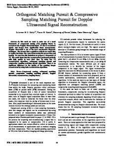
It has been noted that the MP algorithm may be derived as a special case of a technique known as Projection Pursuit (c.f. [2]) in the statistics literature. A shortcoming of the Matching Pursuit algorithm in its originally proposed form is that although asymptotic convergence is guaranteed, the resulting approximation after any nite number of iterations will in general be suboptimal in the following sense. Let N < 1,
gives the optimal approximation with respect to the selected subset of the dictionary. This is achieved by ensuring full backward orthogonality of the error i.e. at each iteration Rk f 2 V?k . For the example in Figure 1, OMP ensures convergence in exactly two iterations. It is also shown that the additional computation required for OMP, takes a simple recursive form. We demonstrate the utility of OMP by example of applications to representing functions with respect to time-frequency localized a�ne wavelet dictionaries. We also compare the performance of OMP with that of MP on two numerical examples.
be the number of MP iterations performed. Thus we have NX ?1
fN = Rk f; xnk+1 � xnk+1 : k=0
De ne VN = Spanfxn1 ; : : :; xnN g. We shall refer to fN as an optimal N-term approximation if fN = PVN f, i.e. fN is the best approximation we can construct using the selected subset fxn1 ; : : :; xnN g of the dictionary D. (Note that this notion of optimality does not involve the problem of selecting an \optimal" N-element subset of the dictionary.) In this sense, fN is an optimal N-term approximation, if and only if RN f 2 V?N . As MP only guarantees that RN f ? xnN , fN as generated by MP will in general be suboptimal. The di�culty with such suboptimality is easily illustrated by a simple example in IR2. Let x1, and x2 be two vectors in IR2, and take f 2 IR2, as shown in Figure 1(a). Figure 1(b) is a plot of kRk f k2
2 Orthogonal Matching Pursuit Assume we have the following kth-order model for f 2 H,
f x2
(a)
2π/3
π/8
x1
f=
Normalized Error
1
(b)
0.8
0.4 0.2 20
40
60 Iteration Number
80
100
kX +1
akn+1xn + Rk+1f; with hRk+1 f; xni = 0, n=1 n = 1; : : :k + 1.
(4) Since elements of the dictionary D are not required to be orthogonal, to perform such an update, we also require an auxiliary model for the dependence of xk+1 on the previous xn 's (n = 1; : : :k). Let,
0.6
0 0
k X
akn xn+Rk f; with hRk f; xni = 0; n = 1; : : :k: n=1 (3) The superscript k, in the coe�cients akn, show the dependence of these coe�cients on the model-order. We would like to update this kth -order model to a model of order k + 1,
f=
120
Figure 1: Matching pursuit example in IR2: (a) Dictionary D = fx1; x2g and a vector f 2 IR2
k X
bknxn + k ; with h k ; xni = 0; n = 1; : : :k: n=1 (5) P Thus kn=1 bknxn = PVk xk+1, and k = PV?k xk+1, is the component of xk+1 which is unexplained by fx1; : : :; xkg. Using the auxiliary model (5), it may be shown that the correct update from the kth -order model to the model of order k + 1, is given by akn+1 = akn ? �k bkn; n = 1; : : :; k (6) k +1 and ak+1 = �k ; k f; xk+1i hRk f; xk+1i where �k = hR h k ; xk+1i = k k k2 hRk f; xk+1i : = 2 kxk+1k ? Pkn=1 bkn hxn; xk+1i
xk+1 =
versus k. Hence although asymptotic convergence is guaranteed, after any nite number of steps, the error may still be quite large. 1 In this paper we propose a re nement of the Matching Pursuit (MP) algorithm that we refer to as Orthogonal Matching Pursuit (OMP). For nonorthogonal dictionaries, OMP will in general converge faster than MP. For any nite size dictionary of N elements, OMP converges to the projection onto the span of the dictionary elements in no more than N steps. Furthermore after any nite number of iterations, OMP 1 A simlar di�culty with the Projection Pursuit algorithm was noted by Donoho et.al. [1] who suggested that back tting may be used to improve the convergence of PPR. Although the technique is not fully described in [1] it appears that it is in the same spirit as the technique we present here.
2
Theorem 2.1 For f 2 H, let Rk f be the residuals generated by OMP. Then
It also follows that the residual Rk+1f satis es,
Rkf = Rk+1 f + �k k ; and
2
kRk f k2 = kRk+1f k2 + jhRkkf; xkk2+1ij :
2.1 The OMP Algorithm
k
(i) klim kR f ? PV ? f k = 0: !1 k
(7)
(ii) fN = PVN f; N = 0; 1; 2; : : :.
Proof: The proof of convergence parallels the proof of Theorem 1 in [3]. The proof of the the second property follows immediately from the orthogonality conditions of Equation (3).
The results of the previous section may be used to construct the following algorithm that we will refer to as Orthogonal Matching Pursuit (OMP).
Initialization:
Remarks:
(I) Compute fhRk f; xni ; xn 2 D n Dk g. (II) Find xnk+1 2 D n Dk such that
The key di�erence between MP and OMP lies in Property (iii) of Theorem 2.1. Property (iii) implies that at the N th step we have the best approximation we can get using the N vectors we have selected from the dictionary. Therefore in the case of nite dictionaries of size M, OMP converges in no more than M iterations to the projection of f onto the span of the dictionary elements. As mentioned earlier, Matching Pursuit does not possess this property.
f0 = 0; R0f = f; D0 = f g x0 = 0; a00 = 0; k = 0
�
Rk f; xnk+1 � � sup jhRk f; xj ij ; 0 < � � 1: j
�
(III) If Rk f; xnk+1 < �, (� > 0) then stop. (IV) Reorder the dictionary D, by applying the permutation k + 1 $ nk+1. � that, (V) Compute bkn kn=1, such Pk xk+1 = n=1 bknxn + k and h k ; xni = 0; n = 1; : : :; k: ?2 (VI) Set, akk+1 +1 = �k = k k k hRk f; xk+1i,
2.3 Some Computational Details As in the case of MP, the inner products
fhRk f; xj ig may be computed recursively. For OMP
we may express these recursions implicitly in the formula
hRk f; xj i = hf ? fk ; xj i = hf; xj i ?
akn hxn; xj i : n=1 (8) The only additional computation required for OMP, arises in determining the bkn 's of the auxiliary model (5). To compute the bkn 's we rewrite the normal equations associated with (5) as a system of k linear equations, vk = Ak bk ; (9) where
akn+1 = akn ? �k bkn ; n = 1; : : :; k; and update the model, fk+1 =
kX +1 n=1
akn+1 xn
Rk+1 f = f ?[fk+1 Dk+1 = Dk fxk+1g: (VII) Set k
k X
vk = [hxk+1; x1i ; hxk+1 ; x2i : : :; hxk+1 ; xki]T bk = �bk1 ; bk2; : : :; bkk �T
k + 1, and repeat (I){(VII).
and
2.2 Some Properties of OMP As in the case of MP, convergence of OMP relies on an energy conservation equation that now takes the form (7). The following theorem summarizes the convergence properties of OMP.
2 6
Ak = 664 3
hx1 ; x1i hx2 ; x1i � � � hxk ; x1i hx1 ; x2i hx2 ; x2i � � � hxk ; x2i
.. .. .. ... . . . hx1; xki hx2 ; xki � � � hxk ; xk i
3 7 7 7: 5
Note that the positive constant � used in Step (III) of OMP guarantees nonsingularity of the matrix Ak , hence we may write
0.5
(a)
(10)
k
-1
However, since Ak+1 may be written as �
�
Ak+1 = Av�k v1k ; k
-1.5 -250
(11)
-200
-150
-100
-50
0
50
100
150
200
250
800
900
1000
0
10
(where � denotes conjugate transpose) it may be shown using the block matrix inversion formula that
(a)
� � 1 k b�k ? bk ; 1 = A? k + b A?k+1 (12) ? b�k 1 , and therefore where = 1=(1 ? v�k bk ). Hence A?k+1 bk+1, may be computed recursively using A?k 1 , and bk from the previous step.
-- MP -1
__ OMP
10
-2
10
-3
10
0
100
200
300
400 500 600 Iteration Number
700
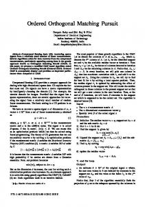
Figure 2: Example I : (a) Original signal f, with OMP approximation superimposed, (b) Squared L2 norm of residual Rk f versus iteration number k, for both OMP (solid line) and MP (dashed line).
3 Examples
Dilation Index
0
In the following examples we consider representations with repect to an a�ne wavelet frame constructed from dilates and translates of the second derivate of a Gaussian, i.e. D = f m;n; m; n 2 ZZg where, m;n (x) = 2m=2 (2m x ? n); and the analyzing wavelet is given by,
-2
-4
-6
-80
-60
-40
-20 0 20 Translation Index
40
60
80
Figure 3: Distribution of coe�cients obtained by applying OMP in Example I. Shading is proportional to squared magnitude of the coe�cients ak , with dark colors indicating large magnitudes.
1=2 ? � (x) = 3p4 � x2 ? 1 e?x2 =2 : Note that for wavelet dictionaries, the initial set of inner products fhf; m;nig, are readily computed by one convolution followed by sampling at each dilation level m. The dictionary used in these examples consists of a total of 351 vectors. In our rst example, both OMP and MP were applied to the signal shown in Figure 2(a). We see from Figure 2(b) that OMP clearly converges in far fewer iterations than MP. The squared magnitude of the coe�cients ak , of the resulting representation is shown in Figure 3. We could also compare the two algorithms on the basis of required computational e�ort to compute representations of signals to within a prespeci ed error. However such a comparison can only be made for a given signal and dictionary, as the number of iterations required for each algorithm depends on both the signal and the dictionary. For example, for the signal of Example I, we see from Figure 4 that it is 3 �
0 -0.5
Normalized L2 Error
bk = A?1 vk :
Original Signal and OMP Approximation 1
�
to 8 times more expensive to achieve a prespeci ed error using OMP even though OMP converges in fewer iterations. On the other hand for the signal shown in Figure 5, which lies in the span of three dictionary vectors, it is approximately 20 times more expensive to apply MP. In this case OMP converges in exactly three iterations.
4 Summary and Conclusions In this paper we have described a recursive algorithm, which we refer to as Orthogonal Matching Pursuit (OMP), to compute representations of signals with respect to arbitrary dictionaries of elementary functions. The algorithm we have described is a modi cation of the Matching Pursuit (MP) algorithm of Mallat and Zhang [3] that improves convergence us4
at each step.
7
10
-- MP __ OMP
Cost (FLOPS)
6
10
Acknowledgements
This research of Y.C.P. was supported in part by NASA Headquarters, Center for Aeronautics and Space Information Sciences (CASIS) under Grant NAGW419,S6, and in part by the Advanced Research Projects Agency of the Department of Defense monitored by the Air Force O�ce of Scienti c Research under Contract F49620-93-1-0085. This research of R.R. and P.S.K was supported in part by the Air Force O�ce of Scienti c Research under contract F49620-92-J-0500, the AFOSR University Research Initiative Program under Grant AFOSR-90-0105, by the Army Research O�ce under Smart Structures URI Contract no. DAAL03-92-G-0121, and by the National Science Foundation's Engineering Research Centers Program, NSFD CDR 8803012.
5
10
4
10
3
10 -2.5
-2
-1.5 Log of Normalized L2 Error
-1
-0.5
Figure 4: Computational cost (FLOPS) versus approximation error for both OMP (solid line) and MP (dashed line) applied to the signal in Example I. 0.4
(a)
0.2
0
-0.2 -250
-200
-150
-100
-50
0
50
100
150
200
References
250
0
[1] D. Donoho, I. Johnstone, P. Rousseeuw, and W. Stahel. The Annals of Statistics, 13(2):496{ 500, 1985. Discussion following article by P. Huber. [2] P. J. Huber. Projection pursuit. The Annals of Statistics, 13(2):435{475, 1985. [3] S. Mallat and Z. Zhang. Matching pursuits with time-frequency dictionaries. Preprint. Submitted to IEEE Transactions on Signal Processing, 1992.
(b)
Normalized L2 Error
10
--- MP ___ OMP
-5
10
-10
10
-15
10
0
10
20
30
40 50 Iteration Number
60
70
80
Figure 5: Example II: (a) Original signal f, (b) Squared L2 norm of residual Rk f versus iteration number k, for both OMP (solid line) and MP (dashed line). ing an additional orthogonalization step. The main bene t of OMP over MP is the fact that it is guaranteed to converge in a nite number of steps for a nite dictionary. We also demonstrated that all additional computation that is required for OMP may be performed recursively. The two algorithms, MP and OMP, were compared on two simple examples of decomposition with respect to a wavelet dictionary. It was noted that although OMP converges in fewer iterations than MP, the computational e�ort required for each algorithm depends on both the class of signals and choice of dictionary. Although we do not provide a rigorous argument here, it seems reasonable to conjecture that OMP will be computationally cheaper than MP for very redundant dictionaries, as knowledge of the redundancy is exploited in OMP to reduce the error as much as possible 5