EVIDENCE ON LEARNING IN COORDINATION GAMES John B. Van Huyck, Raymond C. Battalio, Frederick W. Rankin October 2001 D:\users\inv\el\os5\OS5_3_3.wpd Printed October 12, 2001
Comments to
[email protected] Related research available at http://erl.tamu.edu
Abstract: This paper reports an experiment designed to detect the influence of strategic uncertainty on behavior in order statistic coordination games, which arise when a player’s best response is an order statistic of the cohort’s action combination. Unlike previous experiments using order statistic coordination games, the new experiment holds the payoff function constant and only changes cohort size and order statistic. Key Words: coordination, equilibrium selection, learning, strategic uncertainty, adaptive behavior. JEL classification: c72, c92. Acknowledgments: Alison Aughinbaugh and John Wildenthal provided research assistance. Eric Battalio implemented the experimental design on the TAMU economics laboratory network. The National Science Foundation and Texas Advanced Research Program provided financial support. Any opinions, findings, and conclusions or recommendations expressed in this material are those of the author(s) and do not necessarily reflect the views of the National Science Foundation. © 1996-2001 by the authors. All rights reserved.
I. INTRODUCTION Most situations have multiple mutually consistent ways people can behave. Such situations involve a strategy coordination problem. What is best for a person depends on what others are doing. Strategic uncertainty arises even in situations where objectives, feasible strategies, institutions, and equilibrium conventions are completely specified and are common knowledge. Formally, strategic uncertainty exists whenever a player lacks perfect foresight about what other players are going to do and it influences behavior whenever a player does not have a strictly dominant strategy. Models that do not account for strategic uncertainty may not make accurate predictions about the consequences of environmental changes like group size. This paper reports an experiment designed to detect the influence of strategic uncertainty on behavior in coordination games. The model of strategic uncertainty around which we have organized our thinking is Crawford (1995). The most innovative feature of his model is that “instead of fully endogenizing players’ beliefs and strategy choices (whose differences cannot be traced to differences in players’ information or other characteristics) the model characterizes them statistically, treating certain aspects of the process that describes how they evolve as exogenous parameters to be estimated on a case-by-case basis. This [feature] reflects the conviction ... that it is impossible to predict from rationality alone how people will respond to coordination problems.” He used the data in Van Huyck, Battalio, and Beil (1990, 1991), henceforth VHBB, to estimate the parameters of his model. Once the model has been estimated it can be used to determine the prior probability distribution over equilibria in the underlying coordination game. The new experiment reported below can be seen as an out-of-sample test of his estimated model. Crawford is careful to point out that the estimated behavioral parameters change as payoff functions change. The VHBB (1991) median treatments changed the parameters of the payoff function rather than cohort size and order statistic. The comparison between the VHBB (1991) median treatments and the VHBB (1990) minimum treatments is also confounded by changes in the payoff function. The new experiment holds the payoff function constant and only changes cohort size and order statistic. We focus on three aspects of behavior: subjects’ initial response to the experimental design, which provides evidence on the salience of deductive selection principles; subjects’ adaptive response to their experience in repeated play, which provides evidence on learning theories; and the pattern of equilibrium selection observed in the terminal continuation game, which provides 1
evidence on inductive equilibrium selection theories. The new experiment also uses the ‘blue box’ interface available on the TAMU Economics Laboratory network, which allows a much finer approximation of a continuous action space. Hence, it provides evidence on how important a coarse approximation is for obtaining VHBB’s (1990,1991) results. A finer approximation makes it less costly to explore locally and, hence, may destabilize inefficient mutual best response outcomes. The initial conditions are similar to those observed by VHBB. Increasing the order statistic has a larger impact on initial behavior than increasing group size. Crawford’s model accurately predicts the ordering of the terminal empirical distribution functions. However, we find an anomalous bias towards efficiency that appears to be due to our using a finer approximation of a continuous action space. II. ANALYTICAL FRAMEWORK Van Huyck, Battalio, and Beil (1991,p.893)describe the essential features of the equilibrium selection problem in a many-person decentralized economy and invent a framework to implement those features in a laboratory environment. Here we generalize their framework to include other order statistics along lines suggested in Crawford (1995). Let xi denote the action of player i, where xi 0 X : a compact set of feasible actions. An action combination is the vector of actions x = (x1,...,xn) for the n players. A homogenous action combination occurs when all players take the same action. The jth inclusive order statistic, mj:n, is defined by m1:n # m2:n #...# mn:n, where the mj:n are the xi of action combination x arranged in increasing order. When 1 < j < n, a player contemplating defection from a homogenous action combination can not influence the order statistic. Let the payoff function be such that a player’s unique best response to an action combination is equal to the order statistic mj:n so long as the player can not unilaterally influence the order statistic. Let OS[n,j] denote the stage game of a finitely repeated order statistic game with n players and best response function equal to the expected jth order statistic. This class of order statistic games has the property that any feasible homogenous action combination is a strict equilibrium. Since no payoff function has been specified, it is not possible to apply selection principles based on efficiency or security. However, a simple version of Stahl’s (1993) smartn hierarchy illustrates some interesting properties of order statistic games. Let smart0 players choose according to the uniform distribution on the interval [0,1]. Smart1 players’ best respond 2
to smart0 play. From order statistic theory we know that the order statistic of random variables drawn from a uniform distribution is described by the beta distribution. So the expectation of the order statistic mj:n given smart0 play is x( ' E(mj:n) '
j , n%1
(1)
which would also be a smart1 player’s best response, x*, to his beliefs about the behavior of others in OS[n,j]. Thus, smart1 players increase their action as the order statistic increases and decrease their action as the number of players increase, see equation (1). Let p denote a smart2 players’ perception of the proportion of smart0 players in the population. Smart2 players’ best respond to their perception of p smart0 play and (1-p) smart1 play. This is just x*. Increasing the smartn hierarchy for n > 1 simply reduces the proportion of players who are not giving a best response. A smartn hierarchy has the property that smart0 players, even if they are a minuscule fraction of the population, determine the mutual best response outcome coordinated on by all smartn players with n $ 1 in this class of coordination games.1 Repeated play allows players to learn to coordinate. Consider a repeated OS[n,j] game and let t index time. Crawford (1995) exploits the equivalence of players’ beliefs and best responses in OS[n,j] to develop a model of adaptive dynamics. Following the stochastic control literature, he assumes that player i’s actions and beliefs evolve according to a linear adjustment rule: xi0 ' α0 % ζi0; t > 0, xit ' αt % βt yt&1 % (1&βt) xit&1 % ζit, where y t / m(j:n)t and ζit / εit % ( yt&1 & xit&1) ηit
t > 0.
αt, βt are behavioral parameters. εit, ηit are idiosyncratic random variables distributed with mean 0 and standard deviation σεt, σηt. For simplicity we focus on the constrained model: αt = α and βt = β and
1
Compare Haltiwanger and Waldmann (AER, 1985) on the influence of naive play in situations of strategic complementarity. [Develop]
3
2
2 σεt
'
σε tλ
2
,
2 σηt
'
ση tλ
,
t > 0, where λ is a learning parameter. If λ is
zero, no strategic uncertainty is resolved. Larger values of λ imply more rapid learning. Crawford estimates the behavior parameters of his model using the data reported in VHBB (1990, 1991). Figure 1 graphs the empirical distribution function of the median in period 7 reported in table III of VHBB (1991) and the simulated distribution function reported in table VI of Crawford (1995).2 (The experiment used a coarse grid, which only allowed subjects to choose seven actions indexed 1 to 7: hence, the domain of the graph. When reading the graph it is helpful to know that the empirical distribution function has two mass points of fifty percent each at 4 and 5.) The Kolmogorov goodness-of-fit statistic fails to reject the hypothesis that the empirical distribution function was drawn from the simulated distribution function. Crawford computes the unique solution to his model, provides sufficient conditions for convergence to equilibrium, and makes predictions about the expected change in the order statistic. Given n $ 2, the expected change in the order statistic is negative when j < (n + 1) / 2, zero when j = (n + 1) / 2, and positive when j > (n + 1) / 2. When n is odd, (n + 1) / 2 is the median as in VHBB’s (1991) “average opinion games”. Crawford also proves the following stochastic dominance propositions: Suppose that βt + ηit $ 0 for all i and t, then ceteris paribus increasing j stochastically increases yt and xit for any t; Suppose that βt + ηit $ 0 for all i and t, then ceteris paribus increasing n stochastically decreases yt and xit for any t. The ceteris paribus requirement in the stochastic dominance propositions are problematic and Crawford is careful to point out that the estimated behavioral parameters change as payoff functions change. The VHBB (1991) treatments changed the parameters of the payoff function rather than group size and order statistic. The comparison between the VHBB (1991) median treatments and the VHBB (1990) minimum treatments is also confounded by changes in the payoff function. The new experiment reported below holds the payoff function constant and only changes group size and order statistic.
2
Broseta’s (1993) model gives similar results.
4
III. EXPERIMENTAL DESIGN The payoff function used in this experiment is derived from equation (1) of VHBB (1991): π ( e, m ) ' a m & b ( m & e)2 % c
In VHBB, the action space was e 0 {1,2,...,7}and m was the median. The parameters used for treatment gamma were a = $0.10, b = $0.05, c = $0.70. In the experiment reported here, we used treatment gamma’s parameters, but used a much finer grid over the action space. Specifically, the action space was x 0 {0,1,...,100} and the map used to determine payoffs was e ' 1 % 0.06 x
(2)
Since the sessions were designed to last forty rather than fifteen periods, c was reduced to $0.30. The variable m now denotes the appropriate order statistic: mj:n. Given the payoff function, the equilibria are Pareto ordered with higher actions being associated with more efficient outcomes. The payoff dominant equilibrium, an equilibrium that makes everybody better off compared to all feasible equilibria, is everyone choose 100 for all n and j. The secure equilibrium, an equilibrium in actions that maximize a players payoff in the worst possible outcome, is everyone choose 33 for all n and j.3 Both payoff dominance and security predict the same outcome regardless of cohort size or order statistic. They are examples of solutions that do not account for strategic uncertainty. The treatments in this experiment consist of two cohort sizes of 5 or 7 subjects and two order statistics 2nd or 4th. Figure 2 reports the simulated cumulative distribution function of the order statistic in period 20 for Crawford's constrained model using the parameter estimates for treatment gamma but given the finer grid.4 The simulations maintain the ceteris paribus requirements of the stochastic dominance predictions. None of the
3 This definition defers from maximin in that it is defined for pure rather than mixed strategies and it requires the strategy combination be mutually consistent. 4
The simulated distribution functions are based on 1000 simulations each.
5
OS[7,2] treatments are predicted to converge to the payoff dominant equilibrium, while about 40 percent of the OS[5,4] treatments are predicted to converge to the payoff dominant equilibrium. We chose this design in part based on the large and statistically significant values of the Smirnov statistic for all pairwise comparisons of the treatment variables. Table 1 reports the experimental design matrix. Two games were run simultaneously in the laboratory. This was done to mitigate rumor effects and to allow us to scramble the cohorts at the cross-over between periods 20 and 21. We scrambled the cohorts to mitigate the influence of weak precedents. So, a session consists of two cohorts designated either “A” or “B”. Table 1: Experimental Design Treatment Sessions
Period 1-20
Period 21-40
1A,1B,3A,3B
OS[5,2]
OS[5,4]
4A,4B,5A,5B
OS[5,4]
OS[5,2]
6A,6B,7A,7B
OS[7,2]
OS[7,4]
0A*,0B*,2A, OS[7,4] OS[7,2] 2B,8A,8B * Hardware failure in period 31. It is important to appreciate how we solved the problem of communicating OS[n,j] to undergraduate subjects. We used the ‘blue box’ graphical user interface available in the TAMU Economics Laboratory network.5 The ‘blue box’ interface was first used for the experiment reported in Van Huyck, Cook, and Battalio (1994), which demonstrated its effectiveness. A subject can quickly find his best response to any feasible order statistic by clicking on the ‘blue box’ and moving his mouse up and down until he finds the largest value, which appears next to the line indicating his choice. An experienced user can find his best response in literally two or three seconds. The interface also allows one to check the security level of
5
The “blue box” software has been redone using visual basic and runs in the Economics Research Laboratory (ERL) under Windows NT rather than Novell 3.11.
6
an action just as quickly. The ‘blue box’ interface was enhanced for this experiment to include the history of play on the right side of the screen for easy reference. The bottom of the screen was modified to present a visual representation of order statistics and what it means to change the order statistic. As the subjects went through the instructions on their terminal, an experimenter read them aloud to make the description of the game common information, if not common knowledge. Appendix A reports the instruction text files used. No preplay communication was allowed. Following each repetition of the period game, the relevant summary statistic, which was the only common historical data available to the subjects, appeared on each subject's terminal. After going through the instructions, the subjects filled out a questionnaire, see Appendix A. The questionnaire serves two purposes. First, the questionnaire makes it common information that all subjects can calculate an order statistic and can use the ‘blue box’ interface. Second, the questionnaire frames the game similarly to VHBB, which was run by hand. After the subjects answered the questionnaire correctly, they were given an answer key in the form of a 7×7 matrix. The subjects were undergraduate students attending Texas A&M University and were recruited from economics classes. A total of 110 students participated in this experiment. A session takes less than two hours to conduct and subject earnings averaged more than the minimum wage. If the students had coordinated on the payoff-dominant equilibrium, they could have earned $36. IV. EXPERIMENTAL RESULTS The results are reported in three sections. The first reports initial behavior within a treatment. The second reports adaptive behavior within a treatment and compares behavior with Crawford’s adaptive dynamics. The third reports terminal behavior across treatments, which provides evidence on the predicted stochastic dominance relationships. A. Initial Behavior The data in period 1 are particularly interesting, because they provide evidence on the salience of payoff-dominance and security. Recall that the payoff-dominant equilibrium is all play 100 and the secure equilibrium is all play 33 for all n and j. The payoff dominant action was salient to 22 of 110 subjects or 20 percent of the subjects and the secure action 33 was salient to 3 of 110 subjects or about 3 percent of the subjects. About 67 percent of the subjects choose an action between security and efficiency. 7
As in VHBB (1991), neither payoff-dominance nor security is particularly salient in OS[n,j].6 The median choice overall was 55. The median choice overall in VHBB’s baseline treatment was 4.5 or 58.3 (apply the inverse of the action mapping given in equation 2.) The mean action overall was 62 in both OS[n,j] and VHBB’s baseline treatment. So there exists a sense in which we succeeded in replicating the baseline conditions observed in VHBB despite a much finer action grid, smaller group sizes, and very different experimental methods. Behavior was sensative to strategic uncertainty in that it responds to variations in n and j. An analysis of variance in OS[n,j] rejects the null hypothesis of equal treatment means at conventional levels of statistical significance, see table 2.7 The variation in order statistic and group size influenced behavior in period 1. Inspecting table 2 reveals that subjects react more to differences in order statistic than group size. Table 2: Initial Behavior within Treatments Smartn Predicted Play OS[5,4] 66 OS[7,4] 50 OS[5,2] 33 OS[7,2] 25 Overall F statistic Probability Value
Period 1
Period 21
Pooling Hypotheses
Mean
SD
Mean
SD
F
Prob.
CF
Pro b.
68 69 54 51 62 3.4* 0.02
21 26 25 31 27
60 64 84 60 65 3.3* 0.02
26 24 24 37 31
0.9 0.6 15.3* 0.9
0.35 0.43 0.00 0.33
1.8 1.9 12.3* 3.2
0.78 0.75 0.01 0.53
The order statistic’s influence on initial behavior violates ceteris
6 The corresponding percentages for VHBB’s baseline treatment are 15 percent efficient, 15 percent secure, and 70 percent between security and efficiency. 7
Non-parametric methods also reject pooling across treatments in period 1.
8
paribus assumptions in Crawford’s stochastic dominance propositions. While we didn’t observe the same initial conditions across treatments, the differences in initial treatment means are basically ordered as predicted by the stochastic dominance relationships for terminal outcomes. The propositions continue to be a useful way to think about the data, but some of the behavior predicted to emerge in the session has already be incorporated into initial behavior. An analysis of variance also rejects the null hypothesis of equal treatment means in the initial period of the cross-over treatment: period 21. The mean in OS[n, 4] cross-over treatments in period 21 is lower than in period 1 presumably due to the subjects’ experience in the corresponding OS[n, 2] treatments. The mean in OS[n, 2] cross-over treatments in period 21 is higher than in period 1 again presumably due to experience in the corresponding OS[n, 4] treatments. However, an analysis of variance fails to reject the null hypothesis of equal means in period 1 and period 21 for all treatments except OS[5,2]. In order to test whether the sample distribution functions in period 1 and period 21 are derived from the same population, we used the Epps/Singleton (1986) characteristic function (CF) test, which is based on the Fourier transform of the sample distribution function. The CF statistic fails to reject the null hypothesis that the samples observed in period 1 and period 21 are derived from the same population by treatment except for treatment OS[5,2], see table 2. So we will pool the observations for treatments OS[5,4], OS[7,4], and OS[7,2], when testing the stochastic dominance propositions.8 B. Adaptive Behavior Figures 3 and 4 plot the order statistic by treatment for periods 1-20 and 21-40 respectively. A significant number of cohorts converge to the efficient equilibrium, which was never observed using a coarser approximation of a continuous action space, compare VHBB. Perhaps the most striking examples occur in the ‘average opinion’ treatment: OS[7,4]. Nevertheless, 10 of 18 cohorts fail to converge to 100 in the initial treatment and 11 of 18 cohorts fail to converge to 100 in the crossover treatment. So 58 percent of the cohorts fail to coordinate on the efficient order statistic. Breaking this down by treatment reveals that all of the OS[7,2], three quarters of the initial OS[5,2], half of the OS[7,4], and one
8
Smirnov tests, which are thought to be less powerful in such situations, give the same result.
9
quarter of the OS[5,4] cohorts fail to converge.9 Rather than efficiency, VHBB (1991) found ‘strong precedents’ to be salient. All of the order statistics they observed equaled the order statistic determined in the first period of the treatment. This strong precedent solved their subjects’ coordination problem. Using a finer grid reduces the salience of strong precedents, which was such a striking characteristic of the VHBB data. Restricting attention to the average opinion treatment, half the OS[7,4] cohorts coordinate on the initial median. If one looks at the individual subject data, 26 percent of the subjects play last period’s order statistic in the second period of the OS[7,4] treatments. Crawford’s (1995) model predicts that given n $ 2 the expected change in the order statistic is negative when j < (n + 1)/2, zero when j = (n + 1)/2, and positive when j > (n + 1)/2. Specifically, under the constrained model the expected difference in the order statistic is E(yt & yt&1) ' ((1 & β) σzt&1 % σzt) µj:n,
where σzt denotes the common ex ante standard deviation of the weighted sum of the idiosyncratic innovations ζit and µj:n is the expected value of the jth order statistic of a size n sample of standardized random variables. Note that the sign of the expected innovation is completely determined by µj:n. Following Crawford (1995), we use Teichroew’s (1956) table 1 for the standardized normal distribution to obtain the values of µj:n reported in table 3. Table 3 also reports the average change in the order statistic over the first seven periods by treatment. Two things are striking. First, the average change is small ranging from -0.54 to 2.62. (The sample order statistic changes over the first seven treatment periods range from -7 to 16. A one unit change in VHBB maps into a 17 unit change in the experiment reported here.) Second, all but one of the values is positive. Five of eight are statistically different from zero at the 5 percent level. The average change does not have the predicted sign for all but one of the treatments. Nevertheless, an analysis of variance rejects the null hypothesis of no treatment effects on the average order statistic change.
9
Only one quarter of the cross-over OS[5,2] cohorts fail to converge.
10
Table 3: Average change in order statistic by treatment. Treatment
Average Change in Order Statistic
µj:n
2-7
22-27
OS[5,4]
0.495
1.71*
2.62*
OS[7,4]
0
2.22*
0.83*
OS[5,2]
-0.495
1.42
2.58*
OS[7,2]
-0.757
-0.54
0.55
F statistic 4.42* 2.87* Prob. 0.01 0.04 * Statistically different from zero at 5 percent level. Figure 5 reports one of the most surprising cohorts. The treatment is OS[7,4] and the initial median is 50. The large open circle in the figure denotes the median and the various smaller shapes denote subject choices. The cohort coordinates on a path for the order statistic that increases by 5 for the first eleven periods. The upper bound prevents the cohort from continuing in this way and thereby reintroduces considerable strategic uncertainty. The median falls by 32, which is easily the largest change observed in the experiment. The cohort then coordinates on another time dependent path, but this time increasing by 4. In sum, the average change in the order statistic is influenced by the treatment variables, but not as one would expect based on standard normal innovations. Instead, the distribution of innovations is skewed toward efficiency and this interacting with group size and order statistic results in “creeping” towards efficiency. Sometimes this creeping is perfectly correlated with time. C. Terminal Behavior: Tests for Predicted Stochastic Dominance Ordering. Table 4 reports the initial and terminal order statistic by treatment. An asterisk denotes a mutual best response outcome. Adaptive behavior converges to a mutual best response outcome in 56 percent of the initial cohorts and in 67 percent of the crossover cohorts. Most of the other cohorts have one or two subjects making small deviations from the previous order statistic much like the cohort illustrated in figure 5. Figures for the 11
other cohorts can be found at the ERL web site (erl.tamu.edu). Table 4: Initial and terminal order statistic by treatment. Sessio n
Treatment
1A 1B 3A 3B 4A 4B 5A 5B 6A 6B 7A 7B 0A 0B 2A 2B 8A 8B
OS[5,2] OS[5,2] OS[5,2] OS[5,2] OS[5,4] OS[5,4] OS[5,4] OS[5,4] OS[7,2] OS[7,2] OS[7,2] OS[7,2] OS[7,4] OS[7,4] OS[7,4] OS[7,4] OS[7,4] OS[7,4]
Order Statistic Per. 1 42 35 50 36 78 69 97 95 33 39 6 32 80 50 100 73 50 70
Per. 20 43 40* 100* 36* 100* 80* 100* 100* 27 36 0 33* 100* 50 100* 73 100 100
Cross-over OS[5,4] OS[5,4] OS[5,4] OS[5,4] OS[5,2] OS[5,2] OS[5,2] OS[5,2] OS[7,4] OS[7,4] OS[7,4] OS[7,4] OS[7,2] OS[7,2] OS[7,2] OS[7,2] OS[7,2] OS[7,2]
Order Statistic Per. 21 53 60 67 100 60 48 100* 100 50 50 96 59 33 0 49 15 18 35
Per. 40 53 100* 100* 100* 100* 80* 100* 100* 50 90 100* 59* 31† 0† 49* 15* 46 73*
* denotes mutual best response outcome. † OS in period 31. Figure 6 reports the empirical distribution function of the order statistic in the terminal period of those treatments with initial conditions that did not reject a pooling hypothesis. The basic stochastic dominance relationship predicted is apparent in the data. Increasing the order statistic shifts the empirical distribution function towards more efficient order statistics and increasing group size shifts the empirical distribution function to less efficient order statistics. There are some anomalies. As can be seen by comparing figure 2 and 6, the data reveals a strong bias relative to the dynamic in the direction of efficiency (100). For example, rather than 40 percent of the OS[5,4] treatments converging to the payoff-dominant equilibrium we actually 12
observe almost 80 percent converging. Apparently, subjects focused on the strong precedent of the observed order statistic as in VHBB and then explored locally as in the dynamic. The local exploration was, however, skewed in the direction of efficiency and that led more treatments than predicted to converge to the payoff dominant equilibrium. Let G(x)n:j denote the empirical distribution function observed in the terminal period of treatment OS[n,j]. Smirnov tests of the stochastic dominance hypotheses rejects G(x)5:2 $ G(x)7:2 at the 10 percent level, G(x)5:4 $ G(x)5:2 at the 5 percent level, and G(x)7:4 $ G(x)7:2 at the 1 percent level, see table 5. Hence, there exists significant statistical evidence for the alternative hypothesis that the higher order statistic shifts the mass of the empirical distribution function to more efficient outcomes. The statistical significance of group size is smaller. Table 5: Smirnov Test of Stochastic Dominance Hypotheses. Null Hypothesis T-
Sample Sizes
F(x)5,4 $ G(x)7,4
0.27
F(x)5,2 $ G(x)7,2
Critical Values 0.95
0.99
(8,10)
0.52
0.67
0.60*
(4,10)
0.65
0.80
F(x)7,4 $ G(x)7,2
0.90***
(10,10)
0.50
0.60
F(x)5,4 $ G(x)5,2
0.75**
(8,4)
0.62
0.87
Source: Conover (1980), Table A20, A21. These results allow one to discriminate amongst a number of popular dynamics. Deterministic best-response dynamics, including fictitious play, do not predict the observed order statistic effect. Conversely, any stochastic dynamic that does not allow for the resolution of strategic uncertainty would not predict the observed convergence to mutual best response outcomes. We conclude by reporting a measure of the coordination failure, observed earnings, by treatment. OS[5,4] realized 85 percent, OS[7,4] realized 76 percent, OS[5,2] realized 65 percent, and OS[7,2] realized 58 percent of the maximum feasible earnings. A much finer approximation of a continuous action space does not eliminate the coordination failure 13
observed in order statistic games like those first reported in VHBB (1990,1991). Our subjects’ inability to solve the strategy coordination problem results in significant inefficiencies. D. Sessions that double cohort size: OS[14,4] After the fact, it appears that our simulations overestimated the impact of moving from cohort size 5 to 7. Nevertheless, we believed that the basic intuition--increasing cohort size holding order statistic constant decreases efficiency--was correct. So we conducted four OS[14,4] sessions, which double cohort size. The mean initial choice was 55 with a standard deviation of 27. This is closer to the OS[5,2] and OS[7,2] means of 54 and 51 respectively than to OS[5,4] and OS[7,4] means of 68 and 69 respectively, see table 2. So doubling cohort size has about the same impact on initial behavior as going from the 2nd to 4th order statistic. The terminal order statistics in the four OS[14,4] sessions were 28, 30, 32, and 50. This empirical distribution has exactly the same median as the OS[7,2] distribution, but a narrower range, see figure 6. The differences in the two distributions are not statistically significant. A test of the cohort size stochastic dominance prediction involves a comparison between the OS[7,4] and OS[14,4] empirical distributions. The Smirnov statistic is 0.8, which for sample sizes (4,10) is statistically significant at the one percent level. So we can reject the null hypothesis that F(x)7,4 $ G(x)14,4 and conclude that doubling cohort size holding order statistic constant shifts probability to less efficient outcomes. V. SUMMARY Models that ignore strategic uncertainty can not predict the results of these experiments. Behavior was influenced by both group size and order statistic. Three of four treatment comparisons provide statistically significant differences that are consistent with Crawford’s (1995) stochastic dominance propositions. Changing the order statistic is more powerful than changing group size. The order statistic also influences initial behavior, which exaggerates the stochastic dominance relations. Subjects focus on the observed order statistic and then explore locally. This local exploration is skewed in the direction of efficiency.10 Skewed local exploration interacting with the order statistic causes behavior to slowly creep towards efficiency in some treatments and, most surprisingly,
10
See also Van Huyck, Cook, and Battalio (1993) for similar phenomena.
14
this creeping is perfectly correlated with time in a few treatments. Since this creeping towards efficiency was not observed in VHBB (1991) and three of five initially inefficient OS[7,4] cohorts creep up to the efficient outcome within twenty periods, one must conclude that changing grid size has an important influence on behavior. Reducing the opportunity cost of local exploration increases subjects’ propensity to experiment with actions slightly higher than last period’s order statistic.
15
Cum 1
0.8
0.6
0.4
0.2
e 2
3
4
5
6
7
Figure 1: Empirical distribution function of the median in period 7 reported in table III of Van Huyck, Battalio, and Beil (1991) and simulated distribution function reported in table VI of Crawford (1995).
16
Cum 1
0.8
0.6 OS[7,2]
OS[5,2]
OS[7,4]
OS[5,4]
0.4
0.2
e 20
40
60
80
100
Figure 2: Simulated cumulative distribution function of the order statistic in period 20 for Crawford's (1995) constrained model. OS[i,j] denotes the order statistic game with i subjects and jth order statistic.
17
Figure 3: Order statistic by treatment: period 1-20.
18
Figure 4: Order statistic by treatment: period 21-40.
19
Figure 5: Cohort behavior for session 8A: period 1-20.
20
Cum 1
0.8
0.6
Terminal OS[7,2]
Terminal OS[7,4]
0.4
Terminal OS[5,4] 0.2 Terminal OS[5,2] OS 20
40
60
80
100
Figure 6: Empirical distribution function of the order statistic in the terminal period of those treatments with initial conditions that did not reject the pooling hypothesis.
21
REFERENCES Bruno Broseta, "Strategic Uncertainty and Learning in Coordination Games," UCSD discussion paper, 93-34, August 1993. Bruno Broseta, "Estimation of a Game-Theoretic Model of Learning: An ARCH approach," UCSD discussion paper 93-35, August 1993. Gerard P. Cachon and Colin F. Camerer, "Loss-avoidance and Forward Induction in Experimental Coordination Games," The Quarterly Journal of Economics, 111(1) February 1996. W.J. Conover, Practical Nonparametric Statistics, 2e. (New York, NY: J. Wiley & Sons, 1980). R. Cooper, D.V. DeJong, R. Forsythe, and T.W. Ross, "Selection Criteria in Coordination Games: Some Experimental Results," American Economic Review, 80(1), March 1990. Vincent P. Crawford, "Adaptive Dynamics in Coordination Games," Econometrica 63(1), January 1995, 103-144. Douglas D. Davis and Charles A. Holt, Experimental Economics, (Princeton,NJ: Princeton University Press, 1993). T.W. Epps and Kenneth J. Singleton, “An Omnibus Test for the Two Sample Problem Using the Empirical Characteristic Function,” J. of Statist. Comput. Simul., 26, 1986, 177-203. J. Haltiwanger and M. Waldmann, “Rational Expectations and the Limits of Rationality,” American Economic Review 75(3), June 1985, 326-40. Jack Ochs, "Coordination Problems", Handbook of Experimental Economics, ed. by A. Roth and J. Kagel, 1995. Dale O. Stahl, “Evolution of Smartn Players,” Games and Economic Behavior, 5(4) October 1993, 604-617. D. Teichroew, “Tables of expected values of order statistics and products of order statistics for samples of size twenty and less from the normal distribution.” Annals of Mathematical Statistics, 27, 1956, 410-26. J.B. Van Huyck, R.C. Battalio, and R.O. Beil, "Tacit Coordination Games, Strategic Uncertainty, and Coordination Failure," The American Economic Review 80(1), March 1990, 234-248. J.B. Van Huyck, R.C. Battalio, and R.O. Beil, "Strategic Uncertainty, Equilibrium Selection, and Coordination Failure in Average Opinion Games," The Quarterly Journal of Economics, 106(3), August 1991, 885-911. J.B. Van Huyck, J.P. Cook, and R.C. Battalio, "Adaptive Behavior and Coordination Failure," Journal of Economic Behavior and Organization 32, 1997, 483-503. J.B. Van Huyck, J.P. Cook, and R.C. Battalio, “Selection Dynamics, 22
Asymptotic Stability, and Adaptive Behavior,” Journal of Political Economy, 102(5), October 1994, 975-1005.
23
Appendix A: Instruction Text File for Graphical User Interface: Periods 1 to 20. normal text - OS[7,4] italic text - denotes text that was changed for the other three treatments. INSTRUCTIONS This is an experiment in the economics of strategic decision making. Various agencies have provided funds for this research. If you follow the instructions and make appropriate decisions, you can earn an appreciable amount of money. At the end of today's session, you will be paid in private and in cash. It is important that you remain silent and do not look at other people's work. If you have any questions, or need assistance of any kind, please raise your hand and an experimenter will come to you. If you talk, laugh, exclaim out loud, etc., you will be asked to leave and you will not be paid. We expect and appreciate your cooperation. You will be making choices on a Logitech mouse, which is located on the mouse pad in the middle of your table. You may move the pad to the right or left if this would be more comfortable. Hold the mouse in a relaxed manner with your thumb and little finger on either side of the mouse. Rest your wrist naturally on the table surface. When you move the mouse, let your hand pivot from the wrist. Use a light touch. Your cursor (a white arrow on your screen) should move when you slide the mouse on the mouse pad. If it does not, raise your hand. To participate, you must be able to move the cursor onto an object and click any one of the mouse buttons. We will call pointing at an object and then clicking your mouse "clicking on" an object displayed on the screen. Click on the page down icon located below to display the next page. GENERAL In this experiment you will participate in a market of seven people. At the beginning of period one, each of the participants in this room will be randomly assigned to a group of size seven and will remain in the same group for twenty periods. That is, you will remain grouped with the same six other participants for the next twenty periods. In each period, every participant will pick a value of X. The values of X you may choose are any one of the 101 integers 0, 1, 2, . . . , 98, 99 or 100. The value you pick for X and the value of the 4th order statistic of the X's, (jointly determined by ALL SEVEN participants, including yourself), will determine the payoff you receive for that period. Click on the page down icon to display the next page for a discussion of how to calculate the 4th order statistic. THE 4th ORDER STATISTIC The 4th order statistic is determined as follows. Each period the choices made by all seven participants will be ordered from the smallest to the largest in numerical order. The 4th order statistic for that period is the fourth from the smallest of the ordered choices. To find the fourth order statistic, first (i) arrange the numbers in ascending order and then (ii) counting from the smallest, find the fourth number of the ordered numbers and that is the 4th order statistic. For example, to find the 4th order statistic for the following seven numbers 252, 292, 270, 208, 259, 270, 281 Arrange the numbers in ascending order - c1 c2 c3 c4 c5 c6 c7 208, 252, 259, 270, 270, 281, 292 1 2 3 4 5 6 7
24
Then, counting from the smallest, find the 4th number of the ordered numbers, and that is the 4th order statistic. In this example the 4th order statistic is 270. The 4th order statistic is also identified by 'c4' over the number 270 and '4' under the number 270. MAIN SCREEN We will now view the main screen. You will use the main screen to make your choices each period. While you view the main screen I will read the description of the main screen contained in the next four pages. You can review the text that I am reading at any time during the experiment by returning to the instructions. Click on the word "MAIN" located on the second line down from the top of the screen now. (The second line is the light blue line on your screen). The top line of the main screen displays the current period number, the title of the screen and your current balance. The second line has the word "PROCEED", the abbreviation "INSTR" and the word "RECORD" on it. During the session you will be able to return to these instructions by clicking on "INSTR." You will also be able to view the history of play by clicking on "RECORD", which I will explain in a moment. The remainder of the screen contains: (1) Two blue bars and a ‘blue box’ that will help you understand how your choice and the 4th order statistic influences your earnings each period, (2) A historical record of your past choices, the past 4th order statistics and your earnings for each period of this session, and (3) A bar that represents all seven participant's ordered choices and highlights the 4th order statistic in light blue. Please look at the monitor at the front of the room while I demonstrate how to use the two blue bars and the ‘blue box’ to calculate hypothetical earnings and how to enter your choice each period. Click on the blue bar labelled 4th ORDER STATISTIC and notice that the mouse cursor is replaced by a yellow vertical line and that a yellow vertical line also appears in the ‘blue box’. Immediately below the ‘blue box’ the current value that you have chosen for the hypothetical 4th order statistic appears as a yellow number. Directly below the value for the hypothetical 4th order statistic are three yellow question marks, ???. The question marks are there to remind you that you DO NOT select the 4th order statistic. During the experiment the 4th order statistic will be jointly determined each period by ALL SEVEN participants in your group. By moving your mouse left and right you can select any value between 0 and 100 for your choice of the hypothetical 4th order statistic. Click the mouse a second time to select a value for the hypothetical 4th order statistic and to restore the cursor. Now click on the blue bar labelled YOUR CHOICE. Your mouse cursor is replaced by a green horizontal line and a green horizontal line also appears in the ‘blue box’. Immediately to the right of the ‘blue box’ your current choice and your earnings associated with your current choice of X and the current hypothetical 4th order statistic appears in green. By moving your mouse up and down you can read off the earnings associated with all of your feasible choices and the currently selected hypothetical 4th order statistic. Click the mouse a second time to select a value for your choice and to restore the cursor. Now click again on the blue bar labelled 4th order statistic. By moving the mouse left and right you can read off the earnings associated with all of the possible values for the 4th order statistic and your currently selected choice of X. However, remember that the during the experiment the 4th ORDER STATISTIC is jointly determined by the values of X chosen by ALL SEVEN participants. Your actual payoff will only correspond to a hypothetical payoff if the actual 4th order statistic corresponds to the hypothetical 4th order statistic. Now click the mouse to select a value and to restore the cursor. Now click on the blue square. Notice that moving the mouse here lets you change both YOUR CHOICE of X and the hypothetical value of the 4th ORDER STATISTIC. Click the mouse a second time to select a value and to restore the cursor. In summary, the difference in the three active boxes is in what they control. Clicking on the horizontal bar allows you to change the hypothetical value of the 4th order statistic,
25
while leaving the value of your choice unchanged. Clicking on vertical bar allows you to change the value of your choice by moving its green line up or down with the mouse while leaving the hypothetical value of the 4th order statistic unchanged. Clicking on the blue box allows you to change both values simultaneously. The four columns on the right side of the screen contain the period number, under the label 'Per', a history of your past choices, under the label 'Your Choice', the value of past 4th order statistics, under the label '4th Order Statistic', and your earnings for each past period, under the label 'Your Earnings". When the history fills all of the available lines, only the most recent lines will be displayed. You may use the page up, page down, line up and line down icons at the bottom to review the earlier records. At the bottom of the main screen is a representation of the ordered participant's choices, in order from smallest to largest (c1, c2, c3, c4, c5, c6, c7). The 4th order statistic is highlighted in light blue and enclosed with a light ‘blue box’. The number 4 is also highlighted in blue. When you are ready to enter a choice for a period you do so by clicking on "PROCEED", located on the second line of the main screen. Click on "PROCEED" now and notice that the message 'DO YOU WANT TO PROCEED' in appears in yellow. To proceed you click on the word "YES", in green at the right side of the line. If you want to change your choice at this point you would click on the word "NO", in red. Click on "NO" now and notice that the choice you had entered is canceled and you must now make another choice to proceed. Now click on the blue square. Click the mouse a second time to select a value and to restore the cursor. Click on "PROCEED" now. If you click on "YES" your choice for the period will be entered. Please click on "YES" now to return to the instructions. WAITING SCREEN During a session a waiting screen will appear after you have made a choice. While you are waiting, you can use the two blue bars and the ‘blue box’ to perform hypothetical calculations that will help you understand how your choice and the 4th order statistic influences your earnings each period, similar to the calculations that you can make on the main screen. NOTICE: the vertical line, your choice and earnings and the horizontal line and hypothetical value for the 4th order statistic are ALL IN YELLOW. This color coding is to remind you that you have already made your choice and are currently waiting for other participants to make their choices. NOTICE: the second line DOES NOT contain PROCEED. In addition to making hypothetical calculations, you may also view the instructions and the record screen by clicking on "INSTR" or "RECORD." When all participants have made a choice for the current period you will be automatically switched to the outcome screen. The choice displayed on the WAITING SCREEN is the choice that you made during the demonstration of the main screen. You will automatically return to the instructions in twenty seconds. Click on "WAITING" now. OUTCOME SCREEN During a session, after everyone has made their choices, the outcome screen will appear. The outcome screen summarizes what happened each period for ten seconds. Your choice and period earnings will be highlighted in green. The 4th order statistic, jointly determined by all seven participants in your group, will be highlighted in red. At the bottom of the OUTCOME SCREEN the value of the 4th order statistic for the current period will also be shown in light blue with a light blue outline. The number '4' is also highlighted in light blue. During the experiment, after the period 1 outcome screen has been displayed for ten seconds, you will automatically advance to period 2. Your main screen for period 2 will appear and you may then make a choice for period 2 whenever you are ready. After the outcome screen for period 2 has been displayed for ten seconds you will automatically advance to period 3. This will continue for twenty periods.
26
The outcome screen is not active and, therefore, your mouse cursor will not be present while the outcome screen is displayed. Click on "OUTCOME" now. The value displayed on the outcome screen for YOUR CHOICE is the selection that you made earlier during these instructions. Two different values of the 4th order statistic will each be displayed for ten seconds during this demonstration. I have arbitrarily chosen the values of 25 and 75 for the 4th order statistic during these instructions. You will automatically return to the instructions in twenty seconds. RECORD SCREEN The record screen records the period outcomes and updates your earnings balance. The record screen contains all of the information contained in the past history on the MAIN SCREEN and the WAITING SCREEN plus an additional column labelled Balance that has your balance at the end of each period. At the beginning of the first period your balance is zero. At the end of each period your current period earnings will be added to your balance. At the end of this experiment you will be paid your ending balance, (the sum of all of your period earnings), in cash. Click on the word "RECORD" located on the second line down from the top of your screen now. As the experiment proceeds the records for the earlier periods will scroll off the top of the record screen. You may review the earlier records by clicking on the page up, page down, line up and line down icons located at the bottom of the record screen. Click on RETURN to leave the RECORD SCREEN. QUESTIONNAIRE We will now pass out a questionnaire to make sure that all participants understand how to use the two blue bars and the ‘blue box’ and to make sure that all participants know how to calculate the 4th order statistic and their earnings. Please fill out the questionnaire now. Do not put your name on the questionnaire. Raise your hand when you are finished and we will collect it. If there are any mistakes on any questionnaire, I will go over the relevant part of the instructions again. SUMMARY *** At the beginning of period one, each of the participants in this room will be randomly assigned to a group of size seven and will remain in the same group for twenty periods. *** In each period, every participant will pick a value of X. The value you pick for X and the value of the 4th order statistic of the X's, (jointly determined by ALL SEVEN participants, including yourself), will determine the payoff you receive for that period. *** You make a choice by (i) selecting a value between 0 and 100 for X using the blue bars and\or the ‘blue box’, (ii) clicking the mouse a second time, to select your choice and restore your cursor and then (iii) clicking on "PROCEED" and "YES" to enter and confirm your choice for the current period. *** Remember that you can view the instructions or the record screen by clicking on the appropriate word on the light blue bar. *** Your balance at the end of the session, if positive, will be paid to you in private and in cash. If your balance is negative you will be paid zero. Click on the page down icon located below to display the next page. We have completed the instructions. Again, it is important that you remain silent and do not look at other people's work. If you have a question, please raise your hand, and an experimenter will come to assist you. If there are no questions, period one of the experiment will begin.
27
OS[7,4] Questionnaire 4th ORDER STATISTIC
Y O U R C H O I C E
0
17
33
50
67
83
100
0
(1)____________
0.34998
0.30198
_____________
(2)__________
-0.44202
(3)__________
17
0.24798
0.40200
0.45192
0.40398
0.25200
_____________
-0.34002
33
_____________
0.35592
0.49800
0.54798
(7)__________
0.34800
0.09198
50
-0.15000
_____________
0.44598
0.60000
0.64998
0.60198
0.45000
67
(4)____________
-0.04800
0.28992
(6)____________
0.70200
0.75192
_____________
83
-0.94002
-0.38208
_____________
0.40398
0.65592
0.79800
0.84798
100
(5)____________
-0.83802
-0.31002
0.15000
_____________
0.74598
0.90000
4th ORDER STATISTIC
Y O U R C H O I C E
0
17
33
50
67
83
100
0
0.30000
0.34998
0.30198
0.15000
-0.10602
-0.44202
-0.90000
17
0.24798
0.40200
0.45192
0.40398
0.25200
0.01392
-0.34002
33
0.10398
0.35592
0.49800
0.54798
0.49392
0.34800
0.09198
50
-0.15000
0.20598
0.44598
0.6000
0.64998
0.60198
0.45000
67
-0.50802
-0.04800
0.28992
0.54798
0.70200
0.75192
0.70398
83
-0.94002
-0.38208
0.04800
0.40398
0.65592
0.79800
0.84798
100
-1.50000
-0.83802
-0.31002
0.15000
0.50598
0.74598
0.90000
28
QUESTIONNAIRE (Cont'd) (1) Assume the following choices of X are made by the seven participants in a group. Participant P1 P2 P3 P4 P5 P6 P7
Choice of X 88 15 40 72 30 91 21
(a) Arrange the numbers in ascending order. c1
c2
c3
c4
c5
c6
c7
___ 1
___ 2
___ 3
___ 4
___ 5
___ 6
___ 7
(b) Circle the 1st order statistic in (a) above and calculate the earnings for each participant. Participant
Choice of X
Earnings
P1
88
___________
P2
15
___________
P3
40
___________
P4
72
___________
P5
30
___________
P6
91
___________
P7
21
___________
29
Appendix B Instruction Text File for Graphical User Interface: Periods 21 to 40. normal text - OS[5,4] to OS[5,2] italic text - OS[7,2] to OS[7,4] TREATMENT CHANGES There will be twenty periods in this part of the session. At the beginning of period twenty-one, each of the participants in this room will be randomly re-assigned to a group of size five and will remain in the new group for the next randomly re-assigned to a group of size seven and will remain in the new group for the next twenty periods. As before, in each period, every participant will pick a value of X. The value of the 2nd ORDER STATISTIC of the X's chosen by all five participants and YOUR CHOICE of X will continue to determine the payoff you receive for that period.
As before, in each period, every participant will pick a value of X. However now the value of the 6th ORDER STATISTIC of the X's chosen by all seven participants and YOUR CHOICE of X will determine the payoff you receive for that period. All of the labels on the Main Screen, the Waiting Screen, the Outcome Screen and the Record Screen have been changed to reflect the use of the 6th order statistic during the next twenty periods. NOTE: the earnings associated with the various combinations of YOUR CHOICE of X and the 2nd ORDER STATISTIC have been changed. When period twenty-one begins you can use the two blue bars and the blue box to help you understand how your choice and the 2nd order statistic influences your earnings each period. In addition, the earnings associated with the various combinations of YOUR CHOICE of X and the 6th ORDER STATISTIC have been changed. When period twentyone begins you can use the two blue bars and the blue box to help you understand how your choice and the 6th order statistic influences your earnings each period. THE 6th ORDER STATISTIC The 6th order statistic is determined as follows. Each period the choices made by all seven participants will be ordered from the smallest to the largest in numerical order. The 6th order statistic for that period is the sixth from the smallest of the ordered choices. To find the sixth order statistic, first (i) arrange the numbers in ascending order and then (ii) counting from the smallest, find the sixth number of the ordered numbers and that is the 6th order statistic. For example, to find the 6th order statistic for the following seven numbers 252, 292, 270, 208, 259, 270, 281 Arrange the numbers in ascending order - -
30
c1 c2 c3 c4 c5 c6 c7 208, 252, 259, 270, 270, 281, 292 1 2 3 4 5 6 7 Then, counting from the smallest, find the 6th number of the ordered numbers, and that is the 6th order statistic. In this example the 6th order statistic is 281. The 6th order statistic is also identified by 'c6' over the number 281 and '6' under the number 281. You will start a new record screen. To review the first twenty periods click on "PREVIOUS", which will be located in the upper left corner of the new record screen. Click on "NEXT" to return to the current record screen. The other functions of the record screen work as before. If you have any questions please raise your hand. If there are no questions click on RETURN now.
31