achieve greater autonomy by maintaining consistent and pre- cise reference of the terrain .... on task level autonomy. ..... hard perturbation, HP - 1.0 m and 45â¦.
Overlap-based ICP Tuning for Robust Localization of a Humanoid Robot Simona Nobili, Raluca Scona, Marco Caravagna, Maurice Fallon∗ Abstract— State estimation techniques for humanoid robots are typically based on proprioceptive sensing and accumulate drift over time. This drift can be corrected using exteroceptive sensors such as laser scanners via a scene registration procedure. For this procedure the common assumption of high point cloud overlap is violated when the scenario and the robot’s point-of-view are not static and the sensor’s field-of-view (FOV) is limited. In this paper we focus on the localization of a robot with limited FOV in a semi-structured environment. We analyze the effect of overlap variations on registration performance and demonstrate that where overlap varies, outlier filtering needs to be tuned accordingly. We define a novel parameter which gives a measure of this overlap. In this context, we propose a strategy for robust non-incremental registration. The pre-filtering module selects planar macro-features from the input clouds, discarding clutter. Outlier filtering is automatically tuned at run-time to allow registration to a common reference in conditions of non-uniform overlap. An extensive experimental demonstration is presented which characterizes the performance of the algorithm using two humanoids: the NASA Valkyrie, in a laboratory environment, and the Boston Dynamics Atlas, during the DARPA Robotics Challenge Finals.
I. I NTRODUCTION The primary input to a bipedal locomotion control system is a high frequency estimate of the robot’s state — the 6 degrees-of-freedom (DOF) pose of the robot’s pelvis and its joints configuration. The accuracy of the state estimate is critically important to facilitate effective control and to achieve greater autonomy by maintaining consistent and precise reference of the terrain and objects in the environment. Approaches for state estimation which have been tested on humanoid robots fuse proprioceptive measurements from joint encoders, contact sensors and inertial sensors. Drift in the estimate is reflected by mis-alignment of consecutive point clouds. However, point cloud registration algorithms are highly sensitive to the properties of the input clouds, such as structural features (the presence of planar surfaces), the initial alignment error and the degree of overlap. Overlap is influenced by multiple factors such as the presence of non-static elements in the scene, the viewpoint of the sensor/robot and its field-of-view (FOV). In addition, while the registration of consecutive point clouds leads to accumulated errors, the registration of the current cloud to a common reference prevents accumulated errors but becomes more challenging as the robot moves away from its original pose. Indeed, overlap decreases with the distance from the ∗ The authors are with the Institute of Perception, Action and Behaviour, School of Informatics, University of Edinburgh, UK. {simona.nobili,raluca.scona, marco.caravagna,maurice.fallon}@ed.ac.uk
Fig. 1: The NASA humanoid robot Valkyrie, operating in a laboratory (top). The Boston Dynamics humanoid Atlas during the DRC finals (bottom right, photo credits: MIT team) and the crowded (red box) scenario from the robot’s point of view (bottom left).
pose of the reference point cloud also due to occlusions and non-uniform sampling of the sensor. In this paper we demonstrate how laser-based localization can be combined with a proprioceptive state estimator for a humanoid robot to fulfill the exacting accuracy and robustness requirements described in Section III. We analyze the effect of point cloud overlap variation on the performance of Iterative Closest Point (ICP) alignment. In the case of human-like robots, one of the biggest challenges is introduced by the reduced FOV of the sensors available for exteroception (Figure 2). We define a parameter which describes overlap between two point clouds based on the relative positions of the sensor, the maximum range and the sensor FOV, as well as the distribution of points in the clouds. We propose a strategy for non-incremental 3D scene registration in real environments, called Auto-tuned Iterative Closest Point (AICP). Having first pre-filtered the raw input point clouds to include macro-features such as planes and to implicitly exclude people and clutter, the algorithm automatically tunes the standard ICP outlier filter at run-time using the proposed overlap parameter to define the inlier matches set for the reference and reading clouds1 . We describe the 1 Using the notation from [1], we refer to the ICP inputs as a reference cloud and a reading cloud, the latter to be aligned to the reference.
methods in detail in Section IV. The localization system is evaluated on two full-sized humanoid robots, in Figure 1: the NASA Valkyrie in our laboratory, and the Boston Dynamics Atlas, using a dataset collected by the MIT team during the DARPA Robotics Challenge (DRC) Finals. We present extensive experimental results in Section V, which demonstrate the advantages of flexible outlier-rejection depending on the proposed overlap parameter. II. R ELATED W ORK A. Localization of Humanoid Robots Proprioceptive state estimation for bipedal robots followed from original advances in the field of multi-legged robotics such as Roston and Krotkov [2]. For example, Bloesch et al. [3] first introduced an EKF-based state estimator for a quadruped which Rotella et al. [4] extended for bipedal state estimation. A major focus for humanoids is achieving accurate center of mass (CoM) estimation relative to the supporting feet and accounting for errors in the modeled CoM. Xinjilefu et al. [5] directly estimated this offset using an inverted pendulum model to infer modeling error and/or unexpected external forces. Instead, the approach of Koolen et al. [6] modeled the elasticity of their robot’s leg joints to better distribute error. Our own prior work [7] utilized that elasticity model within a EKF filter to achieve low drift proprioceptive state estimation with the Boston Dynamics Atlas robot. All of these approaches estimate the pelvis pose at high frequency (∼ 500Hz) by combining legs kinematics with IMU data. However these approaches, by their nature, will accumulate incremental drift over time. External sensing is often used to reduce or avoid this drift. Monocular cameras are perhaps the most commonly used exteroceptive sensors, with successful implementations of visual localization including [8] and [9]. In this paper we will instead focus on localization using scanning laser range finders (also known as LIDAR), as vision systems are not as accurate as lasers at long ranges. Hornung et al. [10] initially proposed a laser-based localization method for a NAO robot in a miniature 3D world model with extensions to include observation from a monocular camera presented in [11]. During preparation for the DRC, teams explored using LIDAR to reduce pelvis pose drift as it had a major impact on task level autonomy. In our previous work [7], we computed position measurements relative to a prior map using a rotating 2D laser scan on the Atlas robot. These measurements were integrated into our state estimate using a Gaussian particle filter at the 40Hz frame rate of the LIDAR. Koolen et al. [6] described their approach which instead used lower frequency ICP registration of full 3D point clouds. Both approaches were demonstrated in the laboratory but unfortunately neither method could be used in the DRC Finals due to a lack of field testing and because the arena’s layout contained wide-open spaces with crowds of people. We feel that what was missing was the adaption and tuning of
Fig. 2: The field of view of the Valkyrie’s sensor suite is heavily re-
duced (180◦ ×120◦ ) meaning point clouds are not omni-directional. Most of the LIDAR returns fall on the robot’s head cover. The FOV of Atlas is about 220◦ × 180◦ .
the baseline registration algorithms to these kinds of issues, as well as introspection to detect failures of the registration system. B. Scene Registration The Iterative Closest Point is one of the most commonly used techniques for point cloud registration. Its basic implementation involves the iterative minimization of the pointto-point distances between two point clouds to estimate the relative alignment [12]. Notable improvements to the original algorithm have been introduced in [13] with a point-to-plane error metric better suited for structured environments, and subsequently in [14] and [15]. Alternatively, the Normal Distributions Transform (NDT), introduced in [16], uses standard optimization methods (e.g. Newton’s algorithm) for the alignment. In [17] the authors analyzed the performances of ICP and NDT: although NDT was demonstrated to have a larger valley of convergence, it was found to be less predictable than ICP. ICP makes the implicit assumption that the input point clouds are fully overlapping. This is violated in reality and is typically managed by defining a criteria to identify outliers in the correspondence set (e.g. [18]). Nevertheless, tuning this outlier filter is a critical task for the success of the alignment. III. S YSTEM OVERVIEW AND R EQUIREMENTS The system with the modular configuration of AICP (Section IV) is shown in Figure 3. We present a localization strategy made up of two main components. Firstly, a kinematic-inertial state estimator is used within the closed-loop locomotion controller (either [6] or [7]) and computes a stable but drifting estimate of the robot’s pelvis pose at high frequency (∼ 500Hz). Typical estimation drift is presented in Figure 9 for the continuous walking experiment. Over 200 secs of walking accumulated drift of 10 cm in translation and 5◦ in yaw. Error about the pitch and roll axes is negligible due to the IMU.
Fig. 3: The proposed localization system using AICP. The unfilled arrows indicate the flow of point clouds. We indicate with T the relative transform at each iteration and Ω the overlap parameter.
the comparison of state of the art ICP variants. Their software is publicly available under the name of libpointmatcher3 and will be used as the registration framework in this work. The authors identified two classical ICP variants based on [13] and [19] and use these as their baseline ICP configurations. Their results suggest that the point-to-plane variant, achieves better overall performance than point-topoint. Stable performance can be achieved if the alignment is initialized within a constrained basin of convergence, i.e. 10 cm and 10◦ initial error in 3D translation and rotation, and secondly if the overlap is constantly high while the robot moves in a structured environment. In the following, we discuss the implementation of the AICP algorithm, which overcomes the limitations of the baseline ICP strategies in our real application. A. Pre-filtering
Secondly, the proposed AICP algorithm leverages the low drift state estimator to initialize the alignment to a common reference and properly filter the current point cloud. It updates the state estimate with a correction computed with respect to the global coordinate frame. This assumes that a reference cloud was first captured at the start of operation with the robot observing most of the scene in which we want to localize. Both of the robots involved in our experiments use the Carnegie Robotics Multisense SL as their primary sensing unit, composed of a stereo camera and a Hokuyo UTM30LX-EW planar laser — 40 scans per second with 30 m range — spinning about the forward-facing axis. Every 6 secs the laser spins half a revolution and a 3D point cloud is accumulated. The FOV is however occluded by a protective cover over the robot’s head meaning that a single point cloud typically comprises approximately 100,000 points from the forward facing hemisphere. The speed of rotation of the device (5RPM) is chosen so as to densely sample the terrain when walking. On a parallel thread, the correction is produced with a computation time of about 1 sec. The proprioceptive estimator produces a high rate, low latency estimate without discontinuities while the exteroceptive registration can allow discontinuities (at a low rate) but aims to avoid global drift. The main requirements we identify for such a localization system are (1) accuracy close to 1 − 2 cm on average in position and below 1◦ in orientation, (2) reliability in real semi-structured environments, and (3) registration to a single reference point cloud2 while supporting large translation offsets of as much as 14 m (∼ half the sensor range) and the resulting decrease in overlap, as in Figure 10. IV. ROBUST L OCALIZATION The ICP algorithm has 4 main phases: pre-filtering, data association, outlier filtering and error minimization (Figure 3). Pomerleau et al. [1] proposed a modular implementation of the ICP chain to provide the user with a protocol for 2 For operational simplicity we do not consider building a continuously expanding map using SLAM in this work.
We observe that the alignment of non-uniform point clouds is mainly influenced by denser regions (usually in proximity of the sensor). However, for the alignment to be successful surfaces at different distances should give a balanced contribution to the optimization process. Our pre-filtering approach is divided in two main phases. First, the two input point clouds are uniformly downsampled using a voxel filter [21] (the leaves size is set to 8 cm in our case). Second, we extract planar macro-features such as walls and large surfaces because: • Planar surfaces are represented by a locally regular distribution of points, therefore in the case of slightly incorrect matching, the wrongly associated points still have a good chance of behaving like the correct ones. • People and clutter are implicitly filtered-out. We adopt a region growing strategy for plane segmentation [21]. A region is accepted only if it satisfies criteria about its planarity and dimensions (e.g. larger than 0.30 × 0.30 m). This makes the filtering suitable for man-made environments at least. Figure 4 shows an input cloud before and after the pre-filtering phases. At this stage the remaining point cloud is uniform and has been filtered of clutter points, people in the environment, as well as small and irrelevant regions of the cloud, which as a result do not contribute to the alignment. A comparison between our filter chain and the baseline ICP is presented in Table I. B. Auto-tuned ICP Including false data association matches is a common cause of ICP registration failure. Where points fall on people moving in the scene, on objects outside of the reading cloud’s FOV or which are occluded by other parts of the scene, no successful correspondence can be found and these points will then generate false matches. The standard outlier filter is intended to reject false matches according to a criteria such as a maximum allowed distance or a fixed quantile of the distribution of closest points. For example [19] retains 70% of closest points in 3 https://github.com/ethz-asl/libpointmatcher
Step Reference pre-filtering
Baseline ICP MinDist RandomSampling SurfaceNormal MinDist RandomSampling
Description keep points beyond 1m random down-sampling, keep 10% normals extraction keep points beyond 1m random down-sampling, keep 5%
Data association
KDTree
Outlier filtering
TrimmedDist
Error minimization
PointToPlane
matching with approximation factor � = 3.16 (from [20], [1]) keep 70% closest points (fixed ratio = 0.7) point-to-plane
Reading pre-filtering
AICP Down-sampling RegionExtraction SurfaceNormal Down-sampling RegionExtraction OverlapParam KDTree AutoTrimmedDist PointToPlane
Description uniform down-sampling region growing plane segment. normals extraction uniform down-sampling region growing plane segment. compute Ω matching with approximation factor � = 3.16 (from [20], [1]) keep auto-tuned percentage of closest points (ratio depends on Ω) point-to-plane
TABLE I: Comparison between the baseline ICP and the proposed AICP configuration. horizontal FOV θ. In the case of Valkyrie in Figure 2, r = 30 m and θ = 180◦ . We neglect the reduction in the vertical FOV. • i and j the coordinate frames representing the sensor poses from which w P and w Q have been captured respectively. These frames are defined by the transformations i Tw and j Tw . Consider the set j P of points belonging to the reference cloud P , expressed in the coordinate frame of the reading cloud j, as well as the set i Q of points belonging to Q expressed in i, as: Fig. 4: Pre-filtering. Top: raw point cloud from Valkyrie’s dataset, people are circled in red. Bottom: after pre-filtering. People and small irrelevant features have been filtered-out.
its trimmed outlier filter. We believe that these approaches are too general and produce unsatisfactory performance in practice. Using a fixed parameter assumes constant overlap and this assumption is violated in real scenarios. This is a critical limitation of the baseline ICP solution. Instead we propose to dynamically vary the outlier filter ratio through analysis of the input clouds before registration. Crucially we take advantage of the low drift rate of the kinematic-inertial state estimator. In the following section we define a metric, Ω, to quantitatively represent the overlap between the input clouds. Intuitively, we envisage that the proportion of true matches after data association can be correlated with this overlap metric. In other words: • If overlap is high, the proportion of true matches will be high and could reasonably be approximated by Ω. • If overlap is low, the proportion of true matches will be lower, therefore we need a conservative ratio for the outlier filter, with Ω again being a reasonable approximation. C. Overlap Filter We define Ω by taking into account the initial estimated alignment, range r and field of view θ of the sensor. Being: w • P and w Q the reference and reading clouds respectively, expressed in the world coordinate frame, denoted w. Each cloud is a set of points contained within a subspace of R3 delimited by the sensor range and FOV. We name these subspaces Vi and Vj respectively. Each subspace is a portion of a sphere centered in the sensor pose, with radius r, sectioned by two vertical planes defined by the
j
w
P = j Tw P
i
w
Q = i Tw Q
With each point cloud represented in the coordinate frame of the counterpart, we can determine the subset of these points which lie within the counterpart sensor’s FOV. Sj and Si are then defined as the sets of points living in the volume of intersection between Vi and Vj : ) ( θ p y Sj = ∀p ∈ j P : kpk ≤ r ∧ arctan ≤ ∧ px > 0 px 2 ( ) θ q y i Si = ∀q ∈ Q : kqk ≤ r ∧ arctan ≤ ∧ qx > 0 qx 2 where p = [px , py , pz ]T and q = [qx , qy , qz ]T represent an individual point from each cloud. We define the overlap parameter as |Sj | |Si | Ω= · . |P | |Q| where | • | indicates the cardinality of a set. This metric is so defined under the assumptions that: 1) The pre-filtering strategy described in Section IV-A has removed points belonging to small elements and people in the original point clouds. 2) The initial alignment is within the basin of convergence. In our case, this assumption is satisfied as the drift rate of the state estimator is 1 − 2 cm per step and the correction is computed regularly (every 6 secs). We use Ω to set the outlier filter ratio, with special care for extreme overlap cases: • Where 20% < Ω < 70%, the inlier ratio is set to Ω. • Where Ω < 20%, the inlier ratio is set to 0.20. Generally, at least 20% closest matches are required for alignment optimization.
Features FOV Dynamism Overlap Structure Duration
Scene Area Start Pose K-I SE∗ Vicon
Valkyrie Datasets Reduced (180◦ × 120◦ ) None Exp.A,C: always � 50% Exp.B: from 9% to 100% Structured Exp.A.2: 786 s Exp.B: 1237 s Exp.C.1,C.2: 341 s, 50 s (5.7 × 13.7 × 3.9) m Shown in Figure 1 SE from [6] X
Atlas Dataset Reduced (220◦ × 180◦ ) People, left side Exp.D: decreasing to 10% Semi-structured, right side Exp.D: 1236 s ∼ (14 × 11 × ∞) m Shown in Figure 10 SE from [7] X
TABLE II: Features of the Valkyrie and Atlas datasets. Cells are colored red if the feature reduces the basin of convergence for alignment and green otherwise. *Kinematic-Inertial State Estimator used in the control loop.
Fig. 5: Outlier Filtering. In each image, white points belong to the reference cloud, captured from the blue pose. The red points are accepted inlier matches and the green points are rejected outliers, all belonging to the reading cloud, captured from the yellow pose. Top: ratio = 0.20, Ω = 10%. Bottom: ratio = 0.70, Ω = 10%.
Where Ω > 70%, the inlier ratio is limited to 0.70. Overlap is very high and 70% of the closest points are sufficient for the alignment. This simple relationship between the overlap metric and the outlier ratio results in satisfactory performance in our experiments (Section V). As an illustrative example, Figure 5 (top image) shows the matches preserved in case of low overlap, filtered using a ratio of 0.20, given Ω = 10%. The accepted matches are true matches and as a result the alignment is successful. In contrast, in the lower image an inlier ratio of 0.70 was used and as a result many accepted matches are false and the alignment diverges. •
V. E XPERIMENTAL R ESULTS So as to demonstrate the proposed approach we carried out a series of experiments with the Valkyrie and Atlas robots which correspond to over 60 mins of operation time in total: a) Evaluation of how the proposed approach increases the basin of convergence relative to the baseline ICP approach. b) Exploration of the effect of reducing the overlap between the model and reference point clouds showing that using our prior knowledge of the overlap increases the region of attraction of the core error minimization routine. c) Demonstration of the algorithm running online on the robot where precise localization is essential to approach a target and to climb a set of stairs. d) Finally, a demonstration of performance of the algorithm using a dataset collected at the DARPA Robotics Challenge Finals with the Atlas robot. The algorithm is successful in a semi-structured and crowded environment. The failure of the baseline ICP algorithm in this experiment motivated our work4 . A view of the operation environments is in Figure 1. The relevant features of each dataset are presented in Table II. 4 Additional demonstrations can be viewed at: robotperception.inf.ed.ac.uk/humanoid_estimation
Evaluation Protocol The Valkyrie experiments were carried out in a laboratory with a Vicon motion capture system, used to generate ground truth. For a fair validation of our approach we analyze the performance of the AICP algorithm using the evaluation protocol proposed in [1], namely: 1) AICP is compared to a commonly accepted ICP baseline, which we denote BICP. 2) AICP and BICP are compared on large real world datasets from different environments. 3) Robust statistics are used to produce comparative error metrics. In each case, we compare the estimated pose Pc to the ground-truth robot pose Pg . Being the error ∆P computed as � � ∆R ∆t ∆P = = Pc Pg−1 0 1 the 3D translation error et is defined as the Euclidean distance given the translation vector ∆t: p et = k∆tk = ∆x2 + ∆y 2 + ∆z 2 and the 3D rotation error er is defined as the Geodesic distance given the rotation matrix ∆R: � � trace(∆R) − 1 er = arccos 2 We compare the error distributions using robust statistics (i.e. the quantiles for probabilities 0.50, 0.75, 0.95, which we indicate with Q50, Q75, Q95), which are indicative of accuracy and precision: results are accurate if these quantiles are close to zero, and precise if their difference is small. The choice of error metrics and statistics follows the evaluation convention in [1]. A. Sensitivity to Initial Perturbations As mentioned in Section I, the baseline ICP algorithm is sensitive to initial perturbations (errors in the initial alignment). Here we demonstrate that our proposed prefiltering strategy increases the basin of convergence for AICP, with respect to BICP.
Cumulative Distribution
1 0.8
0.4 0.2 0
Cumulative Distribution
EP, SE + AICP EP, SE + BICP MP, SE + AICP MP, SE + BICP HP, SE + AICP HP, SE + BICP
0.6
0
0.5
1
1.5 2 3D Translation Error [m]
2.5
3
1 0.8 0.6 0.4 0.2 0
0
2
4
6
8 10 12 3D Rotation Error [deg]
14
16
18
20
Fig. 7: Cumulative distribution of translation errors for Valkyrie, Fig. 6: Basin of convergence. An overhead view of the reference cloud is shown at the reference pose (top). Yellow boxes indicate sparse planes in the y direction. We performed tests in a 2 × 2 m basin, with yaw perturbations varying from 0◦ to 90◦ (color scale).
Exp. 1: We select two highly overlapping input clouds (Ω � 70%) and initialize their respective poses with a uniform-grid distribution of perturbations over 3 dimensions, i.e. x, y, yaw as shown in Figure 6. We see that the baseline ICP has a small area of convergence with perturbations of 0.2 m or 10◦ causing the algorithm to fail to properly converge. By comparison, the AICP algorithm is much more robust to perturbations in x and y and rotation in yaw. Successful alignment can be achieved with translation offsets of more than 0.8 m and up to 80◦ in yaw rotation. In particular the pre-filtering strategy enlarges the valley of convergence along the y direction in this case. The main surfaces in this direction are only sampled sparsely due to the range and the axis of rotation of the sensor. In this situation the baseline ICP suffers from a weak contribution to the alignment along this axis. Exp. 2: In their paper Pomerleau et al [1] proposed an experiment in which perturbations are randomly sampled from Gaussian distributions with increasing complexity. In this experiment we present results from such an analysis using 131 samples drawn from each of the following standard deviations: ◦ • easy perturbation, EP - 0.1 m and 10 ◦ • medium perturbation, MP - 0.5 m and 20 ◦ • hard perturbation, HP - 1.0 m and 45 In this experiment the robot continuously walked forward and back. Each new alignment is initialized with a sampled error and the result compared to ground truth. In Figure 7 we show the cumulative distribution of errors for Valkyrie. Not only does AICP outperform the baseline ICP, but it produces reliable alignments in the easy and medium difficulty cases for all the runs. B. Sensitivity to Point Cloud Overlap In Section IV we discussed the importance of properly tuning outlier filtering to account for variations in the point
given easy, medium and hard levels of initial perturbation. The dotted black lines correspond to the quantiles Q50, Q75 and Q95.
cloud overlap — particularly for sensors with limited FOV. Here we evaluate the sensitivity of AICP to variations in the overlap between the inputs. Valkyrie walks and turns in place by approximately 130◦ degrees in each direction. As a result the reading point clouds captured during this run have a large variation in overlap relative to the reference point cloud — between 9% and 100% (top plot, Figure 8) — making the alignment challenging. As mentioned in Section III, corrections from registration are fed back to the state estimate to initialize the next alignment. As a result the initial perturbation is negligible in each alignment and the result is mainly influenced by the current degree of overlap. For the baseline ICP we see that when the overlap falls below 50%, alignment in both rotation and translation fails. In contrast the proposed AICP algorithm is successful throughout by selectively tuning the outlier filter to match the degree of overlap. Robust statistics are provided to demonstrate the distribution of errors (Figure 8). The results show that AICP has the capacity to support non-incremental registration in spite of considerable overlap variations. In turn, non-incremental registration allows recovery from the less accurate alignments (e.g. between seconds 600 − 800). C. Online Integration of AICP In our final Valkyrie experiments we demonstrate integration of the AICP algorithm within our closed loop walking system. These experiments are captured in the video accompanying this paper. Exp. 1: Valkyrie walks repeatedly forward and backward towards a fixed target identified at the beginning of the run. Over the course of the experiment, the median error in translation and rotation estimated by our algorithm are 1.6 cm and 0.4◦ respectively (Figure 9). This satisfies the requirements about expected localization accuracy (requirement 1, Section III). Thanks to this localization performance, the robot reaches the target and maintains a precise pose estimate during the entire run. In contrast, in the case of
Overlap % 3D Rot. Error [deg] 3D Transl. Error [m]
100 50 0 SE + BICP SE + AICP
0.4 0.3
0.2 0.15
0.2
0.1
0.1
0.05
0 10
0 5 4 3
5
2 1
xy Posexy AICP Pose SE
0
0 2 1 0
200
400
600 800 Time [seconds]
1200 B A
1000
0
X: 265
Y: 1.095 Fig. 8:21 Sensitivity to varying input clouds overlap. Boxplots on the
Fig. 10: Sequence of (colored) reading clouds from Atlas dataset aligned to the same reference cloud (white). Overlap is not homogeneous, in order Ω = 60%, 15%, 23%, 10%. Red semi-circles represent the FOV of the robot at each point-of-view.
0.2 0.2
SE SE + AICP
0.15
0.15
0.1
0.1
0.05
0.05
3D Rot. Error [deg]
3D Transl. Error [m]
0 right show the statistics Q50 (tick red bars), Q25 and Q75 (lower and higher end of blue rectangles), Q95 (top end of dashed lines).
0 10
0 6 4
5
2 0
50
100
150 200 Time [seconds]
250
300
A
0
Fig. 9: System integration. The blue line shows the kinematicinertial typical estimation drift while in red we see the corrected estimate from the AICP algorithm.
proprioceptive state estimation only, the robot fails to reach the target repeatedly due to continuous drift. Exp. 2: Valkyrie is placed at 1 m distance from a staircase. The task is to walk towards it and climb up the steps. Planning is performed only once from the starting pose. Over the course of this 50 secs experiment, the median errors in translation and rotation are comparable to Exp. 1. This level of accuracy allows the robot to safely perform the task without needing to re-plan. In contrast, during the DRC robots typically took a few steps at a time to climb stairs or transverse uneven terrain, being paused periodically to manually re-localize and re-plan. In this context, our system was demonstrated to enable greater autonomy in task execution. D. Localization during the DRC Finals In this final experiment we test our algorithm against a dataset collected during a run by the MIT team at the DRC Finals (Pomona, CA, 2015) with the Boston Dynamics Atlas robot. The environment was a semi-structured area of about 14 × 11 m with walls on the right side of the robot and an open-space populated by a crowd of people (walking and sitting) on the left. The robot walks through the test scenario along a 16 m path while passing over uneven terrain and manipulating objects. The scene from Atlas’s point of view
Fig. 11: AICP performance on the DRC Finals dataset with Atlas. Top: a top view of the alignment of 206 point clouds during the run — left: raw clouds with people, right: filtered clouds. Bottom left: state estimation without applying correction, valve perceived in different locations by successive clouds. Bottom right: with successful localization, consistent estimate of the affordance.
at the beginning of the dataset is shown in Figure 1. The presence of many people on the left side of the scenario is a challenge for registration and made localization difficult during the DRC. Corrections from registration are used to update the state estimate and to initialize the next alignment — simulating closed loop integration. The performance of AICP, qualitatively evaluated from careful observation of the map after the run (Figure 11), is such that the computed trajectory is close to error free. People have been filtered-out and do not contribute to the alignment (top right), such that the system satisfies requirement 2. The algorithm is stable and robust enough to compute successful non-incremental alignments during the entire run (with more than 14 m displacement and overlap decreasing to just 10% — as shown in Figure 10), satisfying requirement 3. This experiment is captured in the video accompanying the paper. Figure 12 shows the kinematic-inertial state estimator [7]
3D Transl. Error [m] Overlap %
100 50
R EFERENCES
[1] F. Pomerleau, F. Colas, R. Siegwart, and S. Magnenat, “Comparing ICP variants on real-world data sets,” Autonomous Robots, vol. 34, no. 3, pp. 133–148, Apr. 2013. SE [2] G. P. Roston and E. Krotkov, “Dead reckoning navigation for walking SE + BICP 0.4 robots,” Robotics Institute, Pittsburgh, PA, Tech. Rep. CMU-RI-TR0.4 91-27, Nov. 1991. [3] M. Bloesch, M. Hutter, M. Hoepflinger, S. Leutenegger, C. Gehring, 0.2 0.2 C. D. Remy, and R. Siegwart, “State estimation for legged robots consistent fusion of leg kinematics and IMU,” in Proc. of Robotics: 0 0 Science and Systems (RSS), July 2012. 10 [4] N. Rotella, M. Bloesch, L. Righetti, and S. Schaal, “State estimation 15 for a humanoid robot,” in Proc. of the IEEE/RSJ International Conference on Intelligent Robots and Systems (IROS), 2014, pp. 952–958. 10 X. Xinjilefu, S. Feng, and C. G. Atkeson, “Center of mass estimator [5] 5 for humanoids and its application in modelling error compensation, 5 fall detection and prevention,” in Humanoids, IEEE-RAS International Conference on Humanoid Robots, 2015. 0 0 0 200 400 600 800 1000 1200 SE B [6] T. Koolen, S. Bertrand, G. Thomas, T. de Boer, T. Wu, J. Smith, J. Englsberger, and J. Pratt, “Design of a momentum-based control Time [seconds] framework and application to the humanoid robot Atlas,” International Fig. 12: Atlas at the DRC. The blue line shows the kinematicJournal of Humanoid Robotics, vol. 13, no. 1, 2016. [7] M. Fallon, M. Antone, N. Roy, and S. Teller, “Drift-free humanoid inertial estimation drift while in black we see the corrected estimate state estimation fusing kinematic, inertial and LIDAR sensing,” in Hufrom the baseline ICP algorithm, which diverges at about 400 secs. manoids, IEEE-RAS International Conference on Humanoid Robots, Note that the SE errors are computed against AICP. Nov. 2014. [8] O. Stasse, A. J. Davison, R. Sellaouti, and K. Yokoi, “Real-time 3D and the baseline ICP with errors computed against AICPSLAM for humanoid robot considering pattern generator information,” in Proc. of the IEEE/RSJ International Conference on Intelligent based localization. The baseline ICP fails for overlap less Robots and Systems (IROS), Oct 2006, pp. 348–355. than 50% and demonstrates to be unreliable for complex [9] P. F. Alcantarilla, O. Stasse, S. Druon, L. M. Bergasa, and F. Dellaert, scene registration. Its strategy is unsatisfactory as it adopts “How to localize humanoids with a single camera?” Autonomous Robots, vol. 34, no. 1, pp. 47–71, 2013. no specific measures to deal with the presence of people and A. Hornung, K. M. Wurm, and M. Bennewitz, “Humanoid robot loto explicitly take advantage of the few structures available [10] calization in complex indoor environments,” in Proc. of the IEEE/RSJ in the scene. International Conference on Intelligent Robots and Systems (IROS), Oct. 2010. VI. C ONCLUSIONS [11] S. Oßwald, A. Hornung, and M. Bennewitz, “Improved proposals for highly accurate localization using range and vision data,” in Proc. of In this paper, we proposed an algorithm for robust and the IEEE/RSJ International Conference on Intelligent Robots and accurate scene registration, which we name Auto-tuned ICP. Systems (IROS), Oct. 2012. We explored the degree to which the performance of the ICP [12] P. J. Besl and N. D. McKay, “A method for registration of 3-D shapes,” IEEE Trans. Pattern Anal. Mach. Intell., vol. 14, no. 2, pp. 239–256, algorithm is affected by the overlap between the input point Feb. 1992. clouds, as well as by the magnitude of initial perturbation [13] Y. Chen and G. Medioni, “Object modelling by registration of multiple range images,” Image Vision Comput., vol. 10, no. 3, pp. 145–155, Apr. between them. 1992. We leverage the drifting state estimate derived from our [14] A. Segal, D. Haehnel, and S. Thrun, “Generalized-ICP,” in Proceedhumanoid state estimator [6]-[7] and develop a registration ings of Robotics: Science and Systems (RSS), June 2009. strategy based on careful pre-filtering, adjustment to overlap [15] J. Serafin and G. Grisetti, “NICP: Dense normal based point cloud registration,” in Proc. of the IEEE/RSJ International Conference on variation and non-incremental alignment. The proposed apIntelligent Robots and Systems (IROS), 2015, pp. 742–749. proach increases the basin of attraction of the error minimiza- [16] P. Biber and W. Straer, “The normal distributions transform: a new approach to laser scan matching.” in Proc. of the IEEE/RSJ Internation step of ICP, allowing us to align to a single reference tional Conference on Intelligent Robots and Systems (IROS), 2003, pp. cloud. Consequently our approach avoids incremental error 2743–2748. and recovers from failures. [17] M. Magnusson, A. Nuchter, C. Lorken, A. J. Lilienthal, and J. Hertzberg, “Evaluation of 3D registration reliability and speed Our algorithm overcomes the weaknesses of the baseline a comparison of ICP and NDT,” in IEEE International Conference on ICP identified in [1] in the context of humanoid localization. Robotics and Automation (ICRA), May 2009, pp. 3907–3912. AICP satisfies all requirements identified in Section III. [18] Z. Zhang, “Iterative point matching for registration of free-form curves and surfaces,” Int. J. Comput. Vision, vol. 13, no. 2, pp. 119–152, Oct. Extensive experiments were demonstrated on two fullsized humanoid robots. Future work will focus on the [19] 1994. D. Chetverikov, D. Svirko, D. Stepanov, and P. Krsek, “The trimmed extension of this solution to a SLAM system with failure iterative closest point algorithm,” in Proc. of the International Conference on Pattern Recognition, vol. 3, 2002, pp. 545–548 vol.3. recognition. [20] F. Pomerleau, S. Magnenat, F. Colas, M. Liu, and R. Siegwart, VII. ACKNOWLEDGMENTS “Tracking a depth camera: Parameter exploration for fast ICP,” in Proc. of the IEEE/RSJ International Conference on Intelligent Robots This research was supported by the Engineering and Physand Systems (IROS), Sept. 2011, pp. 3824–3829. ical Sciences Research Council (EPSRC) and by the School [21] R. B. Rusu and S. Cousins, “3D is here: Point Cloud Library (PCL),” in IEEE International Conference on Robotics and Automation (ICRA), of Informatics, University of Edinburgh. We would like to May 2011. 3D Rot. Error [deg]
0
thank the Humanoid Team at the University of Edinburgh, as well as our collaborators at NASA, IHMC and MIT.