Page 1 Accurate Object Localization in 3D Laser Range Scans

Accurate Object Localization in 3D Laser Range Scans Andreas N¨uchter, Kai Lingemann, Joachim Hertzberg

Hartmut Surmann

University of Osnabr¨uck, Institute for Computer Science Knowledge-Based Systems Research Group Albrechtstraße 28 D-49069 Osnabr¨uck, Germany {nuechter|lingemann|hertzberg}@informatik.uni-osnabrueck.de

Fraunhofer Institute for Autonomous Intelligent Systems (AIS) Schloss Birlinghoven D-53754 Sankt Augustin, Germany [email protected]

Abstract— This paper presents a novel method for object detection and classification in 3D laser range data that is acquired by an autonomous mobile robot. Unrestricted objects are learned using classification and regression trees (CARTs) and using an Ada Boost learning procedure. Off-screen rendered depth and reflectance images serve as an input for learning. The performance of the classification is improved by combining both sensor modalities, which are independent from external light. This enables highly accurate, fast and reliable 3D object localization with point matching. Competitive learning is used for evaluating the accuracy of the object localization.

I. I NTRODUCTION Environment perception is a basic problem in the design of autonomous mobile cognitive systems, i.e., of a mobile robot. A crucial part of the perception is to learn, detect, localize and recognize objects, which has to be done with limited resources. The performance of such a robot highly depends on the accuracy and reliability of its percepts and on the computational effort of the involved interpretation process. Precise localization of objects is the all-dominant step in any navigation or manipulation task. This paper proposes a new method for the learning, fast detection and localization of instances of 3D object classes. The approach uses 3D laser range and reflectance data acquired by an autonomous mobile robot to perceive the 3D objects. The 3D range and reflectance data are transformed into images by off-screen rendering. Based on the ideas of Viola and Jones [25], we built a cascade of classifiers, i.e., a linear decision tree. The classifiers are composed of classification and regression trees (CARTs) and model the objects with their view dependencies. Each CART makes its decisions based on feature classifiers and learned return values. The 3D Scan

Off−Screen rendering

Classification

depth

depth

refl.

refl.

features are edge, line, center surround, or rotated features. Lienhart et. al and Viola and Jones have implemented a method for computing effectivly these features using an intermediate representation, namely, integral image [12], [25]. For learning object classes, a boosting technique, particularly, Ada Boost, is used [6]. After detection, the object is localized using a matching technique. Hereby the pose is determined with six degrees of freedom, i.e., with respect to the x, y, and z positions and the roll, yaw and pitch angles. Finally the quality of the object localization is evaluated by fast subsampling of the scanned 3D data. The resulting approach for object detection is reliable and real-time capable and combines recent results in computer vision with the emerging technology of 3D laser scanners. Fig. 1 gives an overview of the implemented system. II. S TATE OF T HE A RT Common approaches of object detection use information of CCD-cameras that provide a view of the robot’s environment. Nevertheless, cameras are difficult to use in natural environments with changing light conditions. Robot control architectures that include robot vision mainly rely on tracking, e.g., distinctive, local, scale invariant features [18], light sources [11] or the ceilings [5]. Other camera-based approaches to robot vision, e.g., stereo cameras and structure from motion, have difficulties providing navigation information for a mobile robot in real-time. Camera-based systems have problems localizing objects precisely, i.e., single cameras estimate the object distance only roughly using the known object size due to the resolution. Estimating depth with stereo is imprecise either: For robots, the width of the stereo base line is limited

Ray Tracing

Model Matching

Evaluation

Result Visualization

comparing subsampled 3D models



    60 27 36
                 ! "#& $% )(' +* , -0 /.2 1 543 Point Distribution

50

number of points

40 30 20 10

0

0

0.1

0.2

0.3

0.4

0.5 1 2 3 distances [cm]

database Fig. 1. System Overview. After acquiring 3D scans, depth and reflection images are generated. In these images, objects are detected using a learned representation from a database. Ray tracing selects the points corresponding to the 2D projection of the object. A 3D model is matched into these points, followed by an evaluation step.

to small values (e.g., < 20 cm), resulting in a typical z-axis error of about 78 cm for objects at the scanner’s maximum ranging distance of about 8 m. Many current successful robots are equipped with distance sensors, mainly 2D laser range finders [24]. 2D scanners cannot detect 3D obstacles outside their scan plane. Currently a general trend exists to use 3D laser range finders and build 3D maps [2], [19], [22], [23]. Nevertheless, only little work has been done in interpreting the obtained 3D models. In [14] we show how complete scenes, made of several automatically registered 3D scans, are labeled using relations given in a semantic net. Object detection in 3D laser scans from mobile robots was presented in [13]. This approach is extended here: First, CARTs are used for a more sophisticated object detection, second, objects are localized in 3D space using point based matching, and third, the accuracy of the matching is evaluated. In the area of object recognition and classification in 3D range data, Johnson and Hebert use the well-known ICP algorithm [4] for registering 3D shapes into a common coordinate system [10]. The necessary initial guess of the ICP algorithm is done by detecting the object with spin images [10]. This approach was extended by Shapiro et al. [16]. In contrast to our proposed method, both approaches use local, memory consuming surface signatures based on prior created mesh representations of the objects. Furthermore, spin images are not able to model complicated objects, i.e., objects with nonsmooth, or non-producible mesh representation. One of the objects used in this paper, the volksbot [1], is of such a structure (Fig. 9). Besides spin images, several surface representation schemes are in use for computing an initial alignment. Stein and Medioni presented the notion of “splash” to represent the normals along a geodesic circle of a center point, which is the local Gauss map for 3D object recognition with a database [20]. Ashrock et al. proposed a pairwise geometric histogram to find corresponding facets between two surfaces that are represented by triangle meshes [3]. Harmonic maps and their use in surface matching have been used by Zhang and Hebert [26]. Recently, Sun and colleagues have suggested so-called “point fingerprints”: They compute a set of 2D contours that are projections of geodesic circles onto the tangent plane and compute similarities between them [21]. All these approaches take the local geometry of the surfaces into account, i.e., meshes. They have problems coping with unstructured point clouds. III. T HE AUTONOMOUS M OBILE ROBOT K URT 3D A. The Kurt Robot Platform Kurt3D (Fig. 2) is a mobile robot platform with a size of 45 cm (length) × 33 cm (width) × 26 cm (height) and a weight of 15.6 kg, both indoor as well as outdoor models exist. Equipped with the 3D laser range finder, the height increases to 47 cm and the weight increases to 22.6 kg.1 1 Videos of the exploration with the autonomous mobile robot can be found at: http://www.ais.fraunhofer.de/ARC/kurt3D/index.html

Fig. 2. The autonomous mobile robot Kurt3D equipped with the 3D laser range finder as presented at RoboCup 2004. The scanners technical basis is a SICK 2D laser range finder (LMS-200).

Kurt3D’s maximum velocity is 5.2 m/s (autonomously controlled: 4.0 m/s). Two 90W motors are used to power the 6 wheels. Compared to the original Kurt3D robot platform, this current version has larger wheels, where the middle wheels are shifted outwards. Front and real wheels have no tread pattern to enhance rotating. Kurt3D operates for about 4 hours with one battery (28 NiMH cells, capacity: 4500 mAh) charge. The core of the robot is an Intel-Centrino-1400 MHz with 768 MB RAM and a Linux operating system. An embedded 16-Bit CMOS microcontroller is used to control the motor. B. The 3D Laser Scanner The 3D laser range finder (Fig. 2) is built on the basis of a 2D range finder by extension with a mount and a standard servo motor [23]. The 2D laser range finder is attached to the mount in the center of rotation for achieving a controlled pitch motion. The servo is connected on the left side (Fig. 2). The 3D laser scanner operates up to 5h (Scanner: 17 W, 20 NiMH cells with a capacity of 4500 mAh, Servo: 0.85 W, 4.5 V with batteries of 4500 mAh) on one battery pack. IV. D ETECTING O BJECTS

IN

3D L ASER DATA

A. Rendering Images from Scan Data After scanning, the 3D data points are projected by an offscreen OpenGL-based rendering module onto an image plane to create 2D images. The camera for this projection is located in the laser source, thus all points are uniformly distributed and enlarged to remove gaps between them on the image plane. Fig. 9 shows reflectance images and rendered depth images (distances encoded by grey-values) as well as point clouds. B. Feature Detection using Integral Images There are many motivations for using features rather than pixels directly. For mobile robots, a critical motivation is that feature-based systems operate much faster than pixel-based systems [25]. The features used here have the same structure as the Haar basis functions, i.e., step functions introduced by Alfred Haar to define wavelets [8]. They are also used in [12], [15], [25]. Fig. 3 (left) shows the eleven basis features, i.e.,

y x X X

Ir (x,y−2) I r(x,y)

N (x0 , y 0 ).

x0 =0 y 0 =0

The integral image is computed recursively, by the formulas: I(x, y) = I(x, y − 1) + I(x − 1, y) + N (x, y) − I(x − 1, y − 1) with I(−1, y) = I(x, −1) = I(−1, −1) = 0, therefore requiring only one scan over the input data. This intermediate representation I(x, y) allows the computation of a rectangle feature value at (x, y) with height and width (h, w) using four references (see Fig. 3 (right)): F (x, y, h, w)

= I(x, y) + I(x + w, y + h) − I(x, y + h) − I(x + w, y).

For computing the rotated features, Lienhart et. al. introduced rotated summed area tables that contain the sum of the pixels of the rectangle rotated by 45◦ with the bottom-most corner at (x, y) and extending till the boundaries of the image (see Fig. 3 (bottom left)) [12]: Ir (x, y) =

x X

x0 =0

Z QJR QJST R QJR QJR QJR Q R WW Y QJSO XX QJR[ QJSO w SONOQJYOSO QJhNOR QJR[O QJR[OQJSO T T R T R T R W X NO O N O N O N O N W X NPNOPO NPO SOPNPO QJSO QJPNPO QJRWW QJSO NPO QJR QJSO NPO QX JR QJSO NPO QJR QJSTNPNPN R QJR QJR QJR Q R PO R P R P R P R T T T T X N N N N N N NPO SOPNPO PNO PO TQJQJPNPO TPNPO TPNPO TPNPO NPO NPN QJQJSO NPN RR QJQJRRWWW QJQJSO NPN RR QJQJRR QJQJSO NPN RRXXX QJQJRR QJQJSO NPN RR QJQJRR QJQJSSTTPNPNPN RR QJQJRR QJQJRR QJQJRR QQ RR PNO NPO PNO O S O S O S O S O S T T T T NPO N N N N N NPO N PO O P O P O P O P V NPNOPO NPO NPO NPO NPO NPO NPO N PO N QJQJPO N R QJRWWWW QJPO N R QJR QJPO N RX QJR QJPO N RV QJR QJPPNPN RVOQJR QJRVOQJR Q R VOVOV UU UU UU Ir (x−h+w,y+w+h−1)

Fig. 3. Top left: Edge, line, diagonal and center surround features are used for classification. Top right: Computation of feature values F in the shaded region is based on the four upper rectangles. Bottom left: Calculation of the rotated integral image Ir . Bottom right: Four lookups in the rotated integral image are required to compute the feature value of a rotated feature F r .

(a)

(b)

thr. = 0.0008941 −0.5598

thr. = 0.03673

thr. = −0.007196 0.4825

−0.8826

0.8981

thr. = −0.00319 −0.8388 thr. = 0.006154 0.898 −0.6285

Fig. 4. Left: A simple feature classifier with its threshold and return values α and β. Right: A Classification and Regression Tree with 4 splits. According to the specific filter applied to the image input section x, the output of the tree, h(x) is calculated, depending on the threshold values.

x−|x0 −y|

X

N (x0 , y 0 ).

C. Learning Classification Functions

y 0 =0

The rotated integral image Ir is computed recursively, i.e., Ir (x, y) = Ir (x − 1, y − 1) + Ir (x + 1, y − 1) + −Ir (x, y − 1) + N (x, y) + N (x, y − 1) using the start values Ir (−1, y) = Ir (x, −1) = Ir (x, −2) = Ir (−1, −1) = Ir (−1, −2) = 0. Four table lookups are required to compute the pixel sum of any rotated rectangle with the formula: Fr (x, y, h, w)

y

@@ AA@@ AA@@ BBAA@@ CBCB CBCB CBCB ED ED

y+h

?> ?> ?> ?> < =< =
= 0

−1.0

thr. = 0.004609 thr. = 0.0001984

−0.8418

thr. = 0.02425

thr. = 0.005112 −0.9333 thr. = −0.003102−0.9618 −0.7775

0.7674

thr. = 0.07443 −0.7831 0.8709 thr. = 0.0008059 thr. = 0.001583

−0.7034

thr. = 0.003583

−0.5853

thr. = 0.0008175 thr. = 0.001529 −0.9087 0.4048 thr. = −0.0009365

−0.475

−0.8292

0.106

thr. = 0.0007613 −0.9586

thr. = 0.0815

thr. = −0.0006408 −0.04683 thr. = 0.001876

0.1188

Σ h(x) >= 0

D. The Cascade of Classifiers The performance of a single classifier is not suitable for object classification, since it produces a high hit rate, e.g., 0.999, but also a high error rate, e.g., 0.5. Nevertheless, the hit rate is significantly higher than the error rate. To construct an overall good classifier, several classifiers are arranged in a cascade, i.e., a degenerated decision tree. In every stage of the cascade, a decision is made whether the image contains the object or not. This computation reduces both rates. Since the hit rate is close to one, their multiplication results also in a value close to one, while the multiplication of the smaller error rates approaches zero. Furthermore, this speeds up the whole classification process, since large parts of the image do not contain relevant data. These areas can be discarded quickly in the first stages. An overall effective cascade is learned by a simple iterative method. For every stage, the classification function h(x) is learned until the required hit rate is reached. The process continues with the next stage using the correctly classified positive and the currently misclassified negative examples. These negative examples are random image parts generated from the given negative examples that pass the previous stages and thus are misclassified. This bootstrapping process is the most time consuming of the training phase. The number of CARTs used in each classifier may increase with additional stages. Fig. 5 shows an example cascade of classifiers for detecting a volksbot in 2D depth images, whose results are given in Table I.

thr. = 0.00447 thr. = 0.01117

thr. = 0.005157 thr. = 0.009565 −0.6336 0.873 0.6733 −0.8661

Σ h(x) < 0 thr. = 0.002204 thr. = −0.0001653 −0.8998

−0.6897

−0.8644

thr. = −0.0007157

thr. = 6.485e−06

−0.4859 thr. = 0.001461 −0.7255

thr. = −0.001167 −1 0.8453

thr. = −0.007075 thr. = 0.0007423 thr. = 0.000449 thr. = −0.003502 0.1369 0.4517 thr. = 0.000411 0.0663 −0.9504

−0.5938

Σ h(x) >= 0

The learning is based on N weighted training examples (x1 , y1 ), . . . , (xN , yN ), where xi are the images and yi ∈ {−1, 1} the classified output i ∈ {1, . . . , N }. At the beginning of the learning phase, the weights wi are initialized with wi = 1/N . The following three steps are repeated to select simple CARTs until a given detection rate d is reached: 1) Every simple classifier, i.e., a CART, is fit to the data. Hereby the error e is calculated with respect to the weights wi . 2) The best CART ht is chosen for the classification function. The counter t is incremented. 3) The weights are updated with wi := wi · e−yi ht (xi ) and renormalized. PT The final output of the classifier is sign( t=1 ht (x)) > 0, with h(x) the weighted return value of the CART. Next, a cascade based on these classifiers is built.

thr. = −0.0009206 −0.9312

0.08552

thr. = 0.001039 thr. = 0.0003634 thr. = −0.000281 0.04225

−0.8349

thr. = 0.004755

−0.9621

thr. = −0.005518 thr. = 0.0004347 0.6207 0.7672 −0.1671 −0.9293

Fig. 5. The first three stages of a cascade of classifiers to detect the object volksbot. Every stage contains several simple classifier P trees that use Haar-like features with a threshold thr. and return values of h(x). h(x) is determined by the path through the trees.

objects on larger scales, the detector is rescaled. An advantage of the Haar-like features is that they are easily scalable.

as correspondences and calculates the transformation, i.e., rotation and translation (R, t) for minimizing the equation E(R, t)

=

Nm X Nd X

2

wi,j ||di − (Rmj + t)|| ,

i=1 j=1

∝

N 1 X ||mi − (Rdi + t)||2 N i=1

(1)

where Nm and Nd , are the number of points in the model set M or data set D, respectively, and wji are the weights for a point match. The weights are assigned as follows: wji = 1, if mi is the closest point to dj within a close limit, wji = 0 otherwise. It is shown that the iteration terminates in a minimum [4]. In each iteration, the transformation is calculated by the quaternion based method of Horn [9]. The assumption is that the point correspondences are correct in the last iteration step. Finally, the pose of the model corresponds to the one in the data set. C. Evaluating the Match Fig. 6. Object points estimation by ray tracing. Top left: All points inside a detection area are extracted. Top Right and bottom: 3D view. 3D points inside the detector area (viewing cone) are red colored.

Each feature requires only a fixed number of look-ups in the integral image, independent of the scale. Time-consuming picture scales are not necessary to achieve scale invariance. Fig. 9 show examples of the detection. To decrease the false detection rate, we combine the cascades of the depth and reflectance images. There are two possible ways for combining: Either the two cascades run interleaved or serial and represent a logical “and” [13]. The joint cascade decreases the false detection rate close to zero. To avoid the reduction of the hit rate, several different offscreen rendered images are used, where the virtual camera is rotated and the apex angle is changed [13]. V. O BJECT L OCALIZATION A. Object Points Estimation After object detection in a 2D projection the algorithm finds the corresponding 3D points using ray tracing. All 3D points that have been projected into the classified area are retrieved using a special OpenGL projection matrix. Fig. 6 (right) shows a rendering of raytraced 3D points. B. Model Matching After the 3D data (set D) that contain the object is found, a given 3D model from the object database is matched into the point cloud. The model M is also saved as 3D point cloud in the database. The well known iterative closest points algorithm (ICP) is used to find a matching [4]. The ICP algorithm calculates iteratively the point correspondences. In each iteration step, the algorithm selects the closest points

Generally, one is interested in the quality of the matching, i.e., the accuracy of the model pose inside the 3D data. Many application specific tasks require this estimation, e.g., complicated robot navigation tasks. However, the value of the error function (1) does not give this information, since point densities influence this value. Different point densities are the result of the scanning process, i.e., the spherical and continuous measurement of the laser. The scanner emits the laser beams in a spherical way such that the data points close to the source are more dense. A competitive learning technique is used to subsample the model and data set. 1) Competitive Object Learning: In addition to subsampling, goals of competitive object learning are the minimization of the expected quantization error and entropy maximization. A finite set of 3D scan points D is subsambled to the set A = {w1 , w 2 , . . . , w N }. Error minimization is done with respect to the following function: 1 X X ||ξ − w i || , E(D, A) = |D| wi ∈A ξ∈Rc

with the set A of samples and the Voronoi set Rc of unit c, i.e., Rc = {ξ ∈ D|s(ξ) = c} and s(ξ) = arg minc∈A ||ξ − wc ||. Entropy maximization guarantees inherent robustness. The failure of reference vectors, i.e., missing 3D points, affects only a limited fraction of the data. Interpreting the generation of an input signal and the subsequent mapping onto the nearest sample in A as a random experiment which assigns a value x ∈ A to the random variable X, then maximizing the entropy X H(X) = − P (x) log(P (x)) x∈A

is equivalent to equiprobable samples. The following neural gas algorithm learns and subsamples 3D points clouds [7]: i.) Initialize the set A to contain N vectors, randomly from the input set. Set t = 0.

]\]\

40 30 20 10 0

Point Distribution

]\]\

50

0

]\]\ `a`b ]\]\ `a _^_^ ```bbb ]\]\ `a `]\ a _^_^ da ``bb dc `a ]\]\ `a _^_^ cda c^ da dcdc fefe `]\ a ``bb fa efa c`a__^ da `]\ a eea c dcdc effe ` b f cda ``bb fa efa ]\]\ `a ^`a__^ da c^ da `]\ a e e dcdc fefe _ c `b fa

number of points

ghgh jjiji ghgh i

0.1

lklk oanmn pop zyz | ~ lklk oam ra qra q o rqrq ts uv wx {a { y }a a }a{|{ }~} 0.2

0.3

 ‚‚ …aƒ„ƒ …† ‰aˆ‡ˆ‡ Š‰Š €  „ ‰a‹a‰ ‹Œ 0.4

 Ž 



— ˜— ˜a ’‘‘’

”“”“

“””“ ”““” –• ’‘’‘ –•a ’‘ –•a • ”“”“ –•–• –a ’‘’‘

0.5 1 2 3 distances [cm]

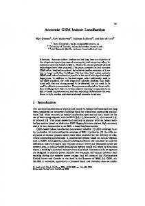
Fig. 8. A typical distribution of distances between closest points after registering two models with a fixed (here: 250) number of points.

Fig. 7. Top: 3D models (point clouds) of the database. Bottom: sumbsampled models with 250 points.

ii.) Generate at random an input element ξ, i.e., select a point from D. iii.) Order all elements of A according to their distance to ξ, i.e., find the sequence of indices (i0 , i1 , . . . , iN −1 ) such that w i0 is the reference vector closest to ξ, w i1 is the reference vector second closest to ξ, etc., w ik , k = 0, . . . , N − 1 is the reference vector such that k vectors wj exists that are closer to ξ than w ik . ki (ξ, A) denotes the number k associated with w i . iv.) Adapt the reference vectors according to ∆wi = ε(t)hλ (ki (ξ, A)) · (ξ − wi ), with the following time dependencies: λ(t)

= λi (λf /λi )t/tmax ,

ε(t) = εi (εf /εi )t/tmax , hλ (k) = exp(−k/λ(t)). v.) Increase the time parameter t. The neural gas algorithms is used with the following parameters: λf = 0.01, λi = 10.0, εi = 0.5, εf = 0.005, tmax = 10000. Note that tmax controls the run time. Fig. 7 shows 3D models of the database (top row) and subsampled versions (bottom) with 250 points. 2) Estimating Matching Quality: Given two registered point sets that contain an equal number of points, e.g., 250 points derived under the premise of minimization of the expected quantization error and entropy maximization, the quality of a matching can be evaluated using the following method: The distribution of shortest distances dij between the

ith and the jth point (closest points) after registering two models with a fixed (here: 250) number of points show a typical structure (Fig. 8). Many distances are very small, i.e., less than 0.3 cm, and there are also many larger distances, e.g., greater than 1 cm. To our experience it is always easy to find a good threshold to separate the two maximas. After dividing the set of distances di , the algorithm computes the mean and the standard deviation of the matching, i.e., v u N0 N0 u 1 X X 1 di σ=t 0 (di − µ)2 µ= 0 N i=1 N i=1 Based on these values one estimates the matching quality by computing a measure D as a function of µ and σ (we have been using D = µ + 3σ). Small values of D correspond to a high quality matching whereas increasing values represent lower qualities. VI. R ESULTS

AND

C ONCLUSION

The process of generating the cascade of classifiers is relatively time-consuming, but it produces quite promising results. The first three stages of a learned cascade are shown in Fig. 5. The time performance of the object detection crucially depends on the bootstrapping, i.e., on the generation of false positive examples during the stage learning. Nevertheless, learning has to be executed only once, the application of the cascade if very fast (300 ms). Thus the major time for the accurate object localization is spent during the model alignment and evaluation step (∼1.4 s). The capabilities of the chosen approach have been evaluated in various experiments. Fig. 9 shows four examples of successful detections and Table I summarizes the object localization results. A. Future Work Needless to say, much work remains to be done. Future work will concentrate on four major aspects: 1) Improve the computational performance of the system to improve robot/environment interaction. 2) Generate high level descriptions and semantic maps including the 3D information, e.g., in XML format.

Fig. 9. Examples of object detection and localization. From Left to right: (1) Detection using single cascade of classifiers. Green: detection in reflection image, yellow: detection in depth image. (2) Detection using the combined cascade. (3) Superimposed to the depth image is the matched 3D model. (4) Detected object in the raw scanner data, i.e., point representation.

TABLE I O BJECT NAME , NUMBER OF STAGES USED FOR CLASSIFICATION VERSUS HIT RATE AND THE TOTAL NUMBER OF FALSE ALARMS USING THE SINGLE AND COMBINED CASCADES . T HE TEST SETS CONSIST OF 89 IMAGES RENDERED FROM 20 3D SCANS . T HE AVERAGE PROCESSING TIME IS ALSO GIVEN , INCLUDING THE RENDERING , CLASSIFICATION , RAY TRACING , MATCHING AND EVALUATION TIME .

object chair kurt robot volksbot robot human

# stages 15 19 13 8

detection rate (reflect. img. / depth img.) 0.767 (0.867 / 0.767) 0.912 (0.912 / 0.947) 0.844 (0.844 / 0.851) 0.961 (0.963 / 0.961)

false alarms (reflect. img. / depth img.) 12 (47 / 33) 0 ( 5 / 7) 5 (42 / 23) 1 (13 / 17)

average proc. time 1.9 sec 1.7 sec 2.3 sec 1.6 sec

The semantic maps will contain spatial 3D data with descriptions and labels. 3) Integrate a camera and enhance the semantic interpretation by fusing color images with range data. The aperture angle of the camera will be enlarged using a pan and tilt unit to acquire color information for all measured range points. 4) Enlarge the database with more objects of an indoor and outdoor environment and build an explicit knowledge base, i.e., specifying a semantic net containing general object relations as well as links to the object database [14]. The final goal of object detection and localization is to develop unrestricted, automatic and highly reliable algorithms that could be used in scenarios like RoboCup Rescue. B. Conclusions This paper has presented a novel method for the learning, fast detection and localization of instances of 3D object classes. The 3D range and reflectance laser scanner data are transformed into images by off-screen rendering. For fast object detection, a cascade of classifiers is built, i.e., a linear decision tree [25]. The classifiers are composed of classification and regression trees (CARTs) and model the objects with their view dependencies. Each CART makes its decisions based on feature classifiers. The features are edge, line, center surround, or rotated features. After object detection the object is localized using a point matching strategy. The pose is determined with six degrees of freedom, i.e., with respect to the x, y, and z positions and the roll, yaw and pitch angles. A final computation returns a quality measure for the object localization. The presented combination of algorithms, i.e., the system architecture enables high accurate, fast and reliable 3D object localization for autonomous mobile robots. R EFERENCES [1] The volksbot robot, http://www.ais.fraunhofer.de/BE/ volksbot/, 2004. [2] P. Allen, I. Stamos, A. Gueorguiev, E. Gold, and P. Blaer. AVENUE: Automated Site Modeling in Urban Environments. In Proceedings of the third International Conference on 3D Digital Imaging and Modeling (3DIM ’01), Quebec City, Canada, May 2001. [3] A. P. Ashrock, R. B. Fisher, C. Robertson, and N. Werghi. Finding surface correspondences for object recognition and registration using pairwise historams. In Proceedings of the European Conference on Computer Vision (ECCV ’98), pages 185 – 201, Freiburg, Germany, June 1998. [4] P. Besl and N. McKay. A method for Registration of 3–D Shapes. IEEE Transactions on Pattern Analysis and Machine Intelligence, 14(2):239 – 256, February 1992. [5] F. Dellaert, W. Burgard, D. Fox, and S. Thrun. Using the Condensation Algorithm for Robust, Vision-based Mobile Robot Localization. In Proceedings of the IEEE Conference on Computer Vision and Pattern Recognition (CVPR ’99), Ft. Collins, USA, June 1999. [6] Y. Freund and R. E. Schapire. Experiments with a new boosting algorithm. In Machine Learning: Proceedings of the 13th International Conference, pages 148 – 156, 1996. [7] B. Fritzke. A growing neural gas network learns topologies. In Advances in Neural Information Processing Systems 7 - Proceedings of the 7th Advances in Neural Information Processing Systems (NIPS ’95), pages 625 – 632, Cambridge, MA, USA, 1995.

[8] A. Haar. Zur Theorie der orthogonalen Funktionensysteme. Mathematische Annalen, (69):331 – 371, 1910. [9] B. Horn. Closed–form solution of absolute orientation using unit quaternions. Journal of the Optical Society of America A, 4(4):629 – 642, April 1987. [10] A. Johnson and M. Hebert. Using spin images for efficient object recognition in cluttered 3D scenes. IEEE Transactions on Pattern Analysis and Machine Intelligence, 21(5):433 – 449, May 1999. [11] F. Launay, A. Ohya, and S. Yuta. Autonomous Indoor Mobile Robot Navigation by detecting Fluorescent Tubes. In Proccedings of the 10th International Conference on Advanced Robotics (ICAR ’01), Budapest, Hungary, August 2001. [12] R. Lienhart and J. Maydt. An Extended Set of Haar-like Features for Rapid Object Detection. In Proceedings of the IEEE Conference on Image Processing (ICIP ’02), pages 155 – 162, New York, USA, Septmber 2002. [13] A. N¨uchter, H. Surmann, , and J. Hertzberg. Automatic Classification of Objects in 3D Laser Range Scans. In Proceedings of the 8th Conference on Intelligent Autonomous Systems (IAS ’04), pages 963 – 970, Amsterdam, The Netherlands, March 2004. [14] A. N¨uchter, H. Surmann, and J. Hertzberg. Automatic Model Refinement for 3D Reconstruction with Mobile Robots. In Proceedings of the 4th IEEE International Conference on Recent Advances in 3D Digital Imaging and Modeling (3DIM ’03), pages 394 – 401, Banff, Canada, October 2003. [15] C. Papageorgiou, M. Oren, and T. Poggio. A general framework for object detection. In Proceedings of the 6th International Conference on Computer Vision (ICCV ’98), Bombay, India, January 1998. [16] S. Ruiz-Correa, L. G. Shapiro, and M. Meila. A New Paradigm for Recognizing 3-D Object Shapes from Range Data. In Proceedings of the IEEE Conference on Computer Vision and Pattern Recognition (CVPR ’03), Madison, USA, June 2003. [17] S. Russell and P. Norvig. Artificial Intelligence, A Modern Approach. Prentice Hall, Inc., Upper Sanddle River, NJ, USA, 1995. [18] S. Se, D. Lowe, and J. Little. Local and Global Localization for Mobile Robots using Visual Landmarks. In Proceedings of the IEEE/RSJ International Conference on Intelligent Robots and Systems (IROS ’01), Hawaii, USA, October 2001. [19] V. Sequeira, K. Ng, E. Wolfart, J. Goncalves, and D. Hogg. Automated 3D reconstruction of interiors with multiple scan–views. In Proceedings of SPIE, Electronic Imaging ’99, The Society for Imaging Science and Technology /SPIE’s 11th Annual Symposium, San Jose, CA, USA, January 1999. [20] F. Stein and G. Medioni. Structural indexing: Efficient 3d object recognition. Transaction on Pattern Analysis and machine Vision (PAMI), 14:125 – 145, February 1992. [21] Y. Sun, J. Paik, A. Koschan, D. Page, and M. Abidi. Point Fingerprint: An New 3D Object Represention Scheme. IEEE transaction on Systems, Man, and Cybernetics — Part B: Cybernetics, 33(4), 2003. [22] H. Surmann, K. Lingemann, A. N¨uchter, and J. Hertzberg. A 3D laser range finder for autonomous mobile robots. In Proceedings of the of the 32nd International Symposium on Robotics (ISR ’01), pages 153 – 158, Seoul, Korea, April 2001. [23] H. Surmann, A. N¨uchter, and J. Hertzberg. An autonomous mobile robot with a 3D laser range finder for 3D exploration and digitalization of indoor en vironments. Robotics and Autonomous Systems, 45(3 – 4):181 – 198, December 2003. [24] S. Thrun, D. Fox, and W. Burgard. A real-time algorithm for mobile robot mapping with application to multi robot and 3D mapping. In Proceedings of the IEEE International Conference on Robotics and Automation (ICRA ’00), San Francisco, CA, USA, April 2000. [25] Paul Viola and Michael J. Jones. Robust real-time face detection. International Journal of Computer Vision, 57(2):137 – 154, May 2004. [26] D. Zhang and M. Hebert. Harmonic maps and their application in surface matching. In Proceedings of the IEEE Conference on Computer Vision and Pattern Recognition (CVPR ’99), pages 2524 – 2530, Ft. Collins, CO, USA, June 1999.

ACKNOWLEDGMENTS The work was done during the authors’ time at the Fraunhofer Institute for Autonomous intelligent Systems. We would like to thank Sara Mitri, Simone Frintrop, Kai Perv¨olz and Matthias Hennig.