In compliance with the Canadian Privacy Legislation some supporting forms may have been removed from this dissertation. While these forms may be included in the document page count, their removal does not represent any loss of content from the dissertation.
PaGrid: A Mesh Partitioner for Computational Grids
by
Sili Huang B.Eng. (CS), Shenzhen University, China, 1999
A Thesis Submitted in Partial Fulfillment of the Requirement for the Degree of
Master o f Computer Science in the Graduate Academic Unit of Computer Science Supervisors:
Eric Aubanel, PhD (Queen's), Computer Science Virendrakumar C. Bhavsar, PhD (I.I.T., Bombay), Computer Science
Examining Board: Bradford G Nickerson, PhD (RPI), Computer Science, Chair Joseph D. Horton, PhD (Waterloo), Computer Science Andrew Gerber, PhD (UNB), Mechanical Engineering
This Thesis is accepted
JDèan of Graduate Studies The University of New Brunswick April 22, 2003 © Sili Huang, 2003
1
*
1
National Library of Canada
Bibliothèque nationale du Canada
Acquisitions and Bibliographic Services
Acquisisitons et services bibliographiques
395 Wellington Street Ottawa ON K1A 0N4 Canada
395, rue Wellington Ottawa ON K1A 0N4 Canada Your file Votre référence ISBN: 0-612-87520-2 Our file Notre référence ISBN: 0-612-87520-2
The author has granted a non exclusive licence allowing the National Library of Canada to reproduce, loan, distribute or sell copies of this thesis in microform, paper or electronic formats.
L'auteur a accordé une licence non exclusive permettant à la Bibliothèque nationale du Canada de reproduire, prêter, distribuer ou vendre des copies de cette thèse sous la forme de microfiche/film, de reproduction sur papier ou sur format électronique.
The author retains ownership of the copyright in this thesis. Neither the thesis nor substantial extracts from it may be printed or otherwise reproduced without the author's permission.
L'auteur conserve la propriété du droit d'auteur qui protège cette thèse. Ni la thèse ni des extraits substantiels de celle-ci ne doivent être imprimés ou aturement reproduits sans son autorisation.
Canada
University ofNew Brunswick HARRIET IRVING LIBRARY This is to authorize the Dean of Graduate Studies to deposit two copies of ray thesis/report in the University Library on the following conditions: (DELETE one of the following condition«) The author agrees that die deposited copies of this thesis/report may be made available to users at the discretion o f the University of New Brunswick OR (b)
The author agrees that the deposited copies ofthis thesis/report may be made available to users only with her/his written permission for the period ending
JUSTIFICATION;
After that date, it is agreed that the thesis/report may be made available to users at the discretion ofthe University of New Brunswick* /4p*nZ
fb b -
\(p> 4)1 = 2, and VB itp r e P lOS z ) I R (p,q) = 2 , *
= fi(A ? ) J i M i = i.
\(p,q)\
The optimal weight for all processors is œ =
Z i ' ,1 ^ and the load balancing condition
for execution time load balancing T, is given by
F , : ^niax -
where 5 is the maximum imbalance factor
(3.5)
We propose to incorporate execution time load balancing to the final partition of the refinement in the uncoarsening phase to refine the load balancing in terms of estimated execution time after the communication cost has been minimized. In order to balance the estimated execution time for each processor, while maintaining the quality of the final partition in terms o f communication cost, all boundary vertices in the final partition are visited in random order and the migrations are sorted in the order of their gains to the
adjacent subdomains.
When the current graph is unbalanced in terms of the estimated execution time, the migrations are allowed if they finally reduce /max of the partition. The vertex migration is made even if the gain is negative. In each iteration, a vertex is visited only once and the iteration repeats until either balance is obtained or no progress in balancing is made.
Example 3.4
Given a 10x10 square mesh with vertex and edge weights equal to 1, and the processor graph as in Figure 3.2 (a) which contains 4 processors, one of the possible partitions is given in Figure 3.4 (a) and it is generated by JOSTLE 3.0. Po
(a) Partitioning without execution time load balancing Figure 3.4
Pi
P2
Pi
(b) Partitioning with execution time load balancing
Execution time load balancing for 10x10 mesh application for Example 3.4.
For the partition shown in Figure 3.4 (a), the total communication cost is 46, and each processor has the same total vertex weight 25. If there is the same ratio R for every processor p in the processor graph, Rp = 0.25, the highest estimated execution time among processors tpi = | npi | + X S l ^ ( v ) l ^ 2 lp 2^ l= 2 5 + 0.25x(12 + 2 x ll) = 33.5 v e z n reP
can then be deduced, and the maximum execution time of this partition is imax = 33.5. Also we can construct the partition in Figure 3.4 (b). The total communication cost is kept at 46, while the partition is relatively more imbalanced than the former partition (in Figure 3.4 (a)) in terms o f the vertex weights assigned to processors, \np0\ = 28 and \n p l1= 23. However, in this partition, the estimated execution time for processors are tpo =28 + 0.25x12 = 31, tpi =24 + 0.25x(12 + 12) = 30, tpi =23 + 0.25x(12 + 22) = 31.5, t
=25 + 0.25x22 = 30.5 , and the maximum execution time is imax =31.5 . This
indicates that the partition may be better in terms of the estimated execution time even though it is imbalanced in terms of the vertex weights assigned to processors.
3.6. Multilevel Partitioning Algorithm In this section, we discuss our implementation of the multilevel graph partitioning algorithm described in Section 3.2. As mentioned, the multilevel partitioning paradigm contains three phases: coarsening, initial partitioning and uncoarsening. Next we describe the implementation of each of these phases.
3.6.1. Coarsening Phase During the coarsening phase, beginning from the original graph Go, a sequence of graphs are constructed; for example, for level /, G, = (Vi, Ei) is generated from a coarsened graph G,./ = (Vj.j, £',./) by finding a maximal matching of G,.y and then collapsing the edges.
Each coarsening level consists of two stages; a matching stage and a contraction stage. It has been shown that the “modified heavy-edge matching” heuristic of METIS, in which a vertex v is matched with another vertex to which it is connected by the heaviest weight, can be beneficial to the optimization [39]. During the matching stage, we follow the “modified heavy-edge matching” heuristic. If more than one edge has the same maximum weight, vertex v will match the vertex u which has the maximum sum of the edge weights to vertex v’s adjacent vertices. In our implementation, two arrays, match and map, are generated in the matching stage. The function match(v) gives the vertex with which v has been matched, and the function coarsen(v) gives the vertex in the coarser graph to which the vertex v is mapped. If during the matching stage vertex v remains unmatched, match(v) = v. Each vertex in the graph is then visited in a random order to find a maximal matching.
During the contraction stage, two matched vertices are collapsed to create a new vertex in the coarser graph. Vertex v and match(v) are collapsed to produce vertex u, i.e. coarsen(v), in the coarser graph with weight \u\ = |vj + |match(v)|. The list of adjacent vertices of u is created from all the adjacent vertices of v and all the adjacent vertices of
match(v), while excluding v and match(v). Let vi, V2 be two vertices that have been matched and coarsen(vi) = coarsen(v2) = u\, the weight of an edge (wi, «2) in the child graph is given by [(m,, u2} | = £ {| {v,,■w) | | coarsen(w) = m2} + £ { | {v2,w}\ Icoarsen(w) = «,}, w
w
where w is a vertex in the parent graph. The iteration of matching and contraction continues until the number of vertices in the coarsest graph equals the number of processors.
3.6.2. Initial Partitioning Phase During the initial partitioning phase, we assign each vertex in the coarsest graph to a different processor while minimizing the cost function (Equation 3.1).
Since there are |P| vertices in the coarsest graph and |P| processors in the processor graph, each edge in £ is a cut edge. Let By = |(v,-, v7)| if v* is adjacent to v7-, while B.j - 0 if v,- is not adjacent to v j , and By = 0 if i = j . We can transform the cost function p
p
(Equation 3.1) to 'P =
in the initial partitioning stage, which leads ;=1 j= \
to a quadratic assignment problem (QAP) [6]. There are many heuristic algorithms addressing this problem. We use an algorithm and its c o ' based on simulated annealing [12], available at the QAP LIB website [6].
3.6.3. Uncoarsening Phase
During the uncoarsening phase, the partition of the coarsest graph is successively
projected back to the original graph Go. At each level, the finer partition of Gi is created from the partition o f G/+; by assigning vertices u and v to the processor to which coarsen(w) = coarsen(v) was assigned at the coarser level. Since the finer graph contains more vertices, even if the partition of G/+/ is at a local minimum from which no migration can be made to improve the total cost, the projected partition of G/ may not be at a local minimum, and G/ has more degrees of freedom to improve the quality of partition. Refinement is performed in each level and the total cost is optimized in each finer graph.
During the refinement stage, the total mapping cost (Equation 3.1) of graph G, is to be minimized while maintaining the load balance of the graph G, with vertex weight load balancing. We have implemented two refinement algorithms: greedy refinement and a variant of KL refinement. For the final uncoarsened graph, execution time load balancing is also implemented.
3.6.3.1. Candidate Processors for Migration
In homogeneous mesh partitioning it is impossible to achieve a positive gain by migrating a vertex to a subdomain to which it is not adjacent. Therefore, most of the partitioners, such as METIS and MiniMax, only consider migration between adjacent subdomains. In heterogeneous mesh partitioning, it is possible to have a positive gain by migrating a vertex to a subdomain to which it is not adjacent [60]. We follow the heuristic suggested by Walshaw and Cross [60], which for a vertex v that was originally assigned to processor p , seeks the maximum gain over a union of processors adjacent to
v in the partition n , together with the processors adjacent to p in the processor graph.
For example, given the processor graph and partitioned application graph shown in Figure 3.5, vertex vi is mapped to processor B and its adjacent subdomain is mapped to processor D. As can be seen in Figure 3.5 (a), processor B is adjacent to processor A, E, and C. To determine the candidate processors for migration, both adjacent subdomains and adjacent processors are considered. So for vertex vi, the candidate processors for migration are processor A, C, D and E.
Figure 3.5
A processor graph and an application graph mapped to it.
Since the input of the mesh partitioner is the mapping cost matrix, the mapping cost matrix has to be transformed to a network graph. We use a breadth-first search technique to search the edges in the mapping cost matrix and rebuild the network graph. The | P | (| P | —1) / 2 edges above the diagonal of the mapping matrix are sorted in order of their weights. Those edges which have the minimum weight among the | P | (| P | -1) / 2
edges are inserted into a queue. Then we conduct the breadth-first technique over the edges in the queue to determine whether the processor graph is connected. If the graph is disconnected after the breadth-first search, the next set of edges are added to the graph. After a connected graph is found, we check whether the connected graph can generate the same network matrix as input. If not, the next set of edges will be added to the queue and the process is repeated until a proper connected graph is recovered.
3.6.3.2. Candidate Vertices for Migration
As stated earlier, it is possible to have a positive gain by migrating a vertex to a subdomain to which it is not adjacent. It is also possible that migration of a vertex v which is not a boundary vertex may generate a positive gain. Therefore, three types of migration candidates are implemented and tested:
(a) all of the vertices, that considers possible migrations of all the vertices in the graph, (b) boundary vertices, that considers only the migrations of the boundary vertices. A boundary vertex refers to a vertex of which one or more edges are cut. For example, given a application graph as Figure 3.5 (b), vertices vi , V2 , and V3 are boundary vertices while vertex V4 is not. (c) boundary+1 vertices, that considers the migrations of the boundary vertices together with the vertices adjacent to the boundary vertices. For example,, given a application graph as Figure 3.5 (b), since vertex V4 belongs to the first level beyond the boundary vertices, it is considered in boundary+1 preference along
3.6.3.3. Imbalance Tolerance
As suggested by Walshaw and Cross [60], a better quality of the partition could be achieved by allowing a large imbalance in the coarsest graphs and then gradually reducing the imbalance in each uncoarsening level. The idea is that allowing a larger amount o f imbalance could lead to a better starting point for the refinement in the next uncoarsening level. Also, it has been shown in [39] that allowing 3% imbalance can improve the quality of partitions. In the refinement stage, we use these heuristics and the formulation from Walshaw and Cross [60], in which for a given level / of uncoarsening, the maximum imbalance is given by
St =
max(l + 2(-==J-)2, 1.03) , / > 0 IK-i I 1.03 ,/=0
3.6.3.4. Bucket Sorting
In our implementation, we use bucket sorting to store and select the gains similar to JOSTLE [59] but with a different bucket tree structure. The bucket sort is an essential tool for the efficient sorting of vertices by their gains.
In order to deal with a large number of vertices, we store buckets in a bucket tree, which is a binary search tree of buckets that are in non-decreasing order of the gains from left to right. The bucket tree structure is depicted in Figure 3.6. Each bucket contains all the
candidate vertices that have the same gain. A bucket is represented by a doubly linked list of bucket items with non-decreasing order of vertex weights. The reason why we sort the candidate vertices in the bucket by vertex weights is that moving vertices with smaller weights earlier can leave more room for other candidate migrations than moving vertices with higher weights earlier. For example, if f ( p , q ) = 2 , we would prefer to move two vertices each o f weight 1 and gain 1 rather than move a vertex of weight 2 and gain 1 .
Figure 3.6
Bucket tree structure.
Each bucket item denotes a candidate vertex and is represented by a linked list with non increasing order of the gains of all its candidate migrations. As we mentioned earlier, the
candidate processors to be considered for a candidate vertex v are not just the processors of adjacent subdomains o f vertex v in the application graph, but also the adjacent processor o f
k
(v )
in the processor graph. Therefore, there can be more than one
candidate migration for a candidate vertex from its original processor to other processors. In cases where there is more than one candidate processor considered for a vertex, if a candidate migration is not acceptable, the other processors still have to be considered. In JOSTLE, a bucket item only stores the first candidate migration of a vertex and when a candidate migration is not accepted, it generates another candidate migration of this vertex to other candidate processors into the bucket tree. Rather than generate the gain each time when a migration of a vertex is not allowed by the load balancing condition, we use a linked list, brother list, to represent a bucket item. A brother list stores all the candidate migrations of a candidate vertex. A brother list is in non-increasing order of the gains and contains a list of brother items. A brother item denotes a candidate migration.
All the candidate vertices are visited in random order, and the vertices having a same gain g are placed together in a bucket ranked as g in the non-decreasing order o f their weights. Thus to find a vertex with maximum gain, we find the bucket with the highest rank in the bucket tree, pick a brother list in this bucket and take out the first brother item in this brother list. If the candidate migration is not allowed by the load balancing condition and the brother list is not empty, the brother list is moved to a bucket with the rank equal to the gain o f the next candidate migration.
Example 3.5 Consider a processor graph given in Figure 3.5 (a) and a portion o f an application graph
shown in Figure 3.5 (b). Consider three vertices vi, V2, and V3. Also suppose vi with weight 2 is in processor B; V2 with weight 4 is in processor D; V3 with weight 4 is in processor F. Vertex vi is in a subdomain adjacent to the subdomain assigned to processor D, V2 is in a subdomain adjacent to the subdomain in processor A, B, E, and V3’s subdomain is adjacent to the subdomain in processor E.
The candidate processors for migration of each vertex are: •
For vj: A, C, D, E
•
For V2 '. A, E, B
•
For V3: E
Suppose the gains for the possible migrations are (the number in parentheses is the gain
of the migration to a particular processor): •
For Vl: A (0), C (-3), D (9), E (2)
•
For v2: A (9), E (0), B(-4)
•
For vj: E (7)
All of the gains are inserted into the bucket tree when the KL algorithm is chosen. Vertices v/ and v2 are placed together in the same bucket ranked 9; since v/ has a smaller weight than v^, vj is placed ahead of v^. Figure 3.7 shows a part of the bucket tree for this example.
3.6.3.5. KL Refinement
The first refinement algorithm we implemented is a variant of the Kemighan-Lin (KL) refinement algorithm, which consists of a limited capability o f hill climbing out of local minima [39, 59]. It has inner and outer iterative loops with the outer loop terminating when no further migrations can be made in the inner loop. The pseudocode of this algorithm based on the above discussion is given in Figure 3.8.
We use two bucket trees (described in Section 3.6.3.4), a candidate tree and an examined tree. The algorithm is initialized by calculating the gains for all candidate vertices as we stated in Section 3.6.3.2, and inserting these candidate vertices into the candidate tree. The initial state o f examined tree is empty. In the inner loop, the candidate vertex with the greatest gain is picked from the candidate tree, and examined to see whether the candidate migration o f the vertex violates the load balancing condition Section 3.5.1.
described in
while (! converged)! /*outer loop*/ converged = true; while (vertices in candidate tree){/*inner loop*/ vertex = best candidate in the tree; if (migration acceptable) { converged = false; migrate vertex { adjust subdomain weights; adjust gains o f adjacent vertices and transfer to appropriate buckets;
} delete it from candidate tree; insert it into examined tree with new gain; if (migration confirmed) { /*hill climbing*/ reset recent move list;
} else{ append vertex to recent move list; if (size o f recent move list > tolerance) break;
} } else if (vertex has more than one candidate migrations) { move to appropriate bucket with second candidate migration
} else{ delete it from candidate tree; insert it into examined tree;
} } for (vertices in recent move list){ migrate vertex back to original subdomain
} for (vertices in candidate tree){ delete it from candidate tree; insert it into examined tree with new gain;
} swap pointers to candidate tree and examined tree;
Figure 3.9
Pseudocode for the KL refinement algorithm.
If this migration is accepted, the vertex is moved to the destination subdomain/processor, the weight of the subdomains/processors and the connectivity of the adjacent vertices are adjusted, the gains are recalculated for the vertex and all of its neighbors and finally the vertex is transferred to the examined tree.
The migrations o f the vertices are confirmed if they improve the quality of the partition; otherwise, the migrations are recorded in a recent move list for further examination. The inner loop terminates when the candidate tree is empty or it may terminate early if the number o f migrations in the recent move list exceeds the tolerance; similar to METIS [39] in our implementation, we have defined this tolerance as 30. Once the inner loop has terminated, all the migrations in the recent move list are undone (if there are any) and the vertices remaining in the candidate tree are transferred to the examined tree. Finally the pointers to the two bucket trees are swapped and ready for the next iteration. The outer loop terminates when there are no migrations allowed or all the migrations that are allowed are undone.
Migration Acceptance
At each refinement stage, all the candidate vertices are visited in random order. For each candidate vertex v, the gain (Equation 3.2) to each processor in the set of candidate processors, even if it is negative, is generated and the candidate vertex is inserted into the bucket tree.
Then we pick the vertex with the greatest gain from the bucket tree and check whether the migration of it satisfies the load balancing condition
. A migration for a candidate
vertex v with weight |v| from processor p to q is accepted for further examination if («) wmax > M , or
(3.6)
(b) wmax
S and |^q| + |v| < co8. Equation (3.6) is an implementation of load balancing con d ition C on d ition (a) states
that if a graph is not yet within the imbalance tolerance, only the migration which reduces the vertex weights of a processor, is allowed. If the partition is already balanced, condition (b) guarantees that the partition cannot be unbalanced again.
After moving vertex v, the algorithm recalculates the gains of the vertices to which vertex v is adjacent in order to reflect the change in the subdomain, and moves or inserts these vertices to the corresponding bucket in the bucket tree. When a migration of vertex v is disallowed, if there are still other candidate processors available, the vertex v with the greatest gain of the rest of candidate migrations is moved to the corresponding bucket in the bucket tree. Once a vertex is moved to the examined tree, it is not considered again for migration in the same iteration.
Migration Confirmation
Let n denote the best partition reached so far, Y represent the best total cost of this partition and wmax denote the maximum processor weight of the partition n . Let n l denote the subsequent partition after I migrations, VF/ represent the total cost of this partition and wlmix denote the maximum processor weight of this partition. The migration is confirmed if one of the following conditions is satisfied (a) ¥ ' < ? , (b) ' F ' ^ a n d v . L , ^ ,
(3.7)
(c) W " m a x > co and Wmax < w r max
v*v
That is, the KL refinement algorithm moves vertex v to a subdomain/processor that
leads to the largest cost reduction without violating the balancing condition. If no cost reduction is possible by moving a vertex v, then v is moved to the subdomain/processor that improves the balance. The algorithm continues moving vertices until there is no migration allowable in an iteration (convergence) or it has performed n vertex migrations that have not decreased the total cost in the case when the partition is already balanced. In the latter case, the last n migrations are undone. Similar to METIS [39], in our implementation n = 30.
3.6.3.6. Greedy Refinement
Greedy refinement is a simplification of the KL refinement, in which the vertex migrations with negative gain are not considered for the refinement once the graph is balanced; therefore the lookahead capability of KL is eliminated.
The lookahead
capability o f the KL algorithm enables the migration of an entire cluster of vertices across a partition boundary. The reason why we eliminate lookahead is that the clusters of vertices are collapsed into a single vertex at successive coarsening phases, thus the migration of a vertex at a coarser level represents the migration of a group of vertices in the original graph. The elimination of lookahead could possibly generate a quality similar to the KL refinement algorithm while saving refinement time.
All the candidate vertices are visited in random order. For each candidate vertex v, the gains of the migrations are generated and the vertex is inserted into the bucket. Then the vertices are picked out of the bucket tree in a non-increasing order of gains. If the partition is balanced, migrations that yield negative gains are not allowed. If the
partition is unbalanced, then migrations with negative gain are allowed. All the allowed candidate migrations are checked whether they satisfy the migration acceptance conditions (Equation 3.2). The migrations that satisfy these conditions are then made. The algorithm converges when there is no more allowable migration.
3.6.3.7. Execution time load balancing
After the iteration of projection and refinement for each coarsening level, the graph is finally projected back to the original graph. As we stated earlier in Section 3.5, there is an opportunity to improve the partition to minimize estimated execution time. Therefore, we propose to add an execution time load balancing stage.
We implement a variant of the KL algorithm, which is similar to the algorithm described in Section 3.6.3.5, except that the migration acceptance condition and the migration confirmation condition are different.
Migration Acceptance
All the candidate vertices that are visited in random order are placed together in the candidate tree according to their gains. For a vertex v assigned to processor p, let fmax denote the new value o f t mx, and tp represent the new value of tp after a migration. For each candidate vertex v, the gain (Equation 3.2) to each processor in the set of candidate processors, even if it is negative, is generated and the vertex is inserted into the bucket
tree. Then we pick the vertex with the greatest gain from the bucket tree and check whether the migration of it satisfies the execution time migration acceptance condition
as follows, which is an implementation of T,. (a)' v
m ax
’
ta q < t„ p and iq < £„, p> or
. .
. .
(3.5)
(b) tmm